Statistical arbitrage is a trading strategy class that uses statistical and econometric techniques to exploit historically related financial instruments’ relative mispricings. Statistical arbitrage trading strategies still work as new instruments, exchanges, and financial markets create trading opportunities.
What Is Statistical Arbitrage?
Statistical arbitrage, also known as stat arb, refers to any trading strategy that uses statistical and econometric techniques to profit with an element of market risk reduction. Arbitrage opportunities occur both in the long-term and short term.
Gerry Bamberger developed the first arbitrage strategy using pair trades trading at Morgan Stanley in the mid-1980s.
The easiest way to understand statistical arbitrage is by example. We’ll start with a simple pairs trading strategy like Gerry Bamberger invented.
The price of gold affects the profitability of gold miners. If the price of gold goes up, gold miners’ profitability should also increase. If the gold price increases quickly, either the gold miner’s stock prices must follow, or the gold price must fall.
See the gold and the gold miner’s ETF price for 2006-07 – 2007-06 below.
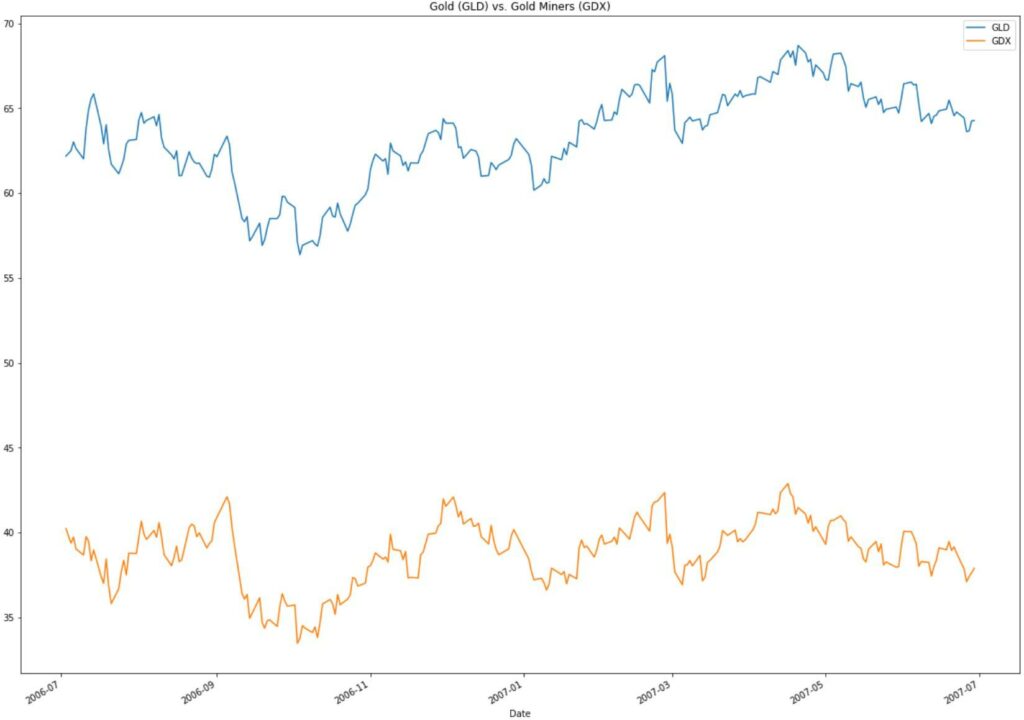
Notice how both prices move together — they are correlated.
When gold prices moved up faster than gold miners, we would sell the gold miners short and buy the gold miners; when gold’s price movements fell more quickly than gold miners, we could buy gold and sell the miners. Going back in time, we could have profited from this relationship with almost zero market risk — meaning if the market went up, down, or sideways, we still made money.
Pairs trading is one of the many types of statistical arbitrage.
Types of Statistical Arbitrage
While there are multiple types of statistical arbitrage, we’ll discuss the most common:
- Market Neutral Arbitrage
- Cross Asset Arbitrage
- Cross Market Arbitrage
Market Neutral Arbitrage
When a strategy has a beta of zero, which means its returns are not affected by the market’s price movement, it’s market-neutral. The pairs trading strategy mentioned above is a market-neutral strategy.
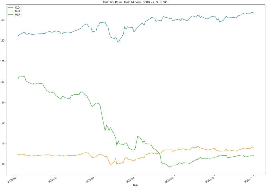
While trading two stocks is the most conceptually simple statistical arbitrage strategy, we’re not limited to only two stocks. Investors can use any number of financial instruments cointegrating; however, there’s only one other with a unique name — We’re trading “triplets” when we arbitrage three assets together.
We can update our pairs strategy and make it a triplet by adding oil. The price of oil is an input into the profitability of gold miners.
Cross Asset Arbitrage
Cross-asset arbitrage is an investment strategy that bets on the price discrepancy between a financial asset and its underlying. This can be an index and its futures, indices and component stocks, or anything where one financial instrument represents another.
Let’s look at an ETF asset arbitrage example.
Based on market capitalization, the Nasdaq 100 Index (NDX) contains the 100 largest domestic and international non-financial companies listed on the Nasdaq Stock Market.
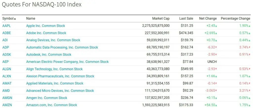
The Invesco Nasdaq ETF (QQQ) tracks the Nasdaq 100 index. What happens if Apple’s price is up by 1.90% on the day, but the ETF fund flows are negative? Invesco will likely need to purchase or sell a disproportionate amount of Apple to keep their ETF weighting representative of the index weighting.
In other words, intelligent statistical arbitrageurs can profit from these imbalances.
Cross Market Arbitrage
Market arbitrage simultaneously buys and sells the same financial instrument in different markets, allowing an astute investor to take advantage of price discrepancies.
Let’s see how we could potentially market arbitrage Bitcoin.
One could buy Bitcoin at the lower price on Coinbase at $34,421 and sell it immediately on Bitfinex for $34,514, making a $93 profit. Now granted, there’s more to it than this, such as exchange risk, slippage, algorithmic trading platforms, etc. But the point remains the same, buy an asset trading at a lower price in one market and sell it for a higher price in another.

Risks of Statistical Arbitrage
Statistical arbitrage models contain both systemic and idiosyncratic investing risks. All use past relationships to predict the future, and these relationships can change based on changes in the economy. Additionally, each type of statistical arbitrage strategy carries strategy risk. Also, securities that stop cointegrating can cointegrate once again.
In our pairs example above, between May 23, 2006, and July 14, 2008, gold prices (GLD) and gold miners (GDX) cointegrate with 99% probability. But what seemed like a certainty stopped working. Why?
That brings us to the triplets example — oil prices started to climb, putting pressure on the gold miner’s profitability while simultaneously breaking the pairs trading strategy. Adding oil to the pair improves the results, but nothing is a sure thing in the market — except for maybe taxes and bankruptcies?
Another risk of statistical arbitrage strategies is overconfidence. Going back to our pairs trading example, if it’s cointegrating at 99% probability and you apply leverage, what happens when it stops working seemingly out of nowhere? Don’t be the next Long Term Capital Management.

Additionally, profitable statistical arbitrage strategies are in high demand as who wouldn’t want near riskless profits? The challenge is that once enough players discover the statistical relationship, the profits are often “arbitraged” away.
While the model breaking down is the primary risk, there are many risks with each type of statistical arbitrage.
With pairs trading strategies, a company could go bankrupt or shift its product mix, breaking a pair — I don’t advise pair trading individual stocks but more on that later. Cross-market arbitrage carries a significant exchange default “hack” risk, especially with Bitcoin and other cryptocurrencies. And cross-asset arbitrage contains unique risks such as stock delisting. There is always frequency risk, too. Higher frequency strategies incur significant trading costs and portfolio turnover.
Additionally, while the market risk is reduced from arbitrage strategies, it’s essential to check for correlation between arbitrage strategies, portfolios, and positions during the portfolio construction process.
The best defense to these risks is always to assume the model could fail at any point in time and fully understand each arbitrage strategy’s risks and the overall risks in the context of your portfolios.
Does Statistical Arbitrage Still Work?
While the performance of the more common statistical arbitrage strategies has declined or become non-existent, new statistical arbitrage strategies regularly appear; furthermore, many financial instruments can come in and out of cointegration.
For instance, the previously discussed gold, gold miner, and oil triplet have gone in and out of cointegration.
Let’s take a step back and think about why statistical arbitrage works.
From a market-neutral strategy perspective, there are fundamental economic relationships that hold. We’ve discussed one with the price of gold and gold miners, but there are plenty of others.
This brings me to another point. I’m not particularly eager to pair trade stocks, as I mentioned above. The reason is that the relationships are often tenuous and fall about. Additionally, idiosyncratic risk can obliterate cointegration. Instead, I prefer to trade cointegrating ETFs.
Additionally, anything new generally can be arbitraged. This includes new markets and securities.
Statistical Arbitrage Analysis Techniques
Statistical arbitrage models rely on finding patterns in the data using statistical and mathematical models.
An analyst would typically use either Matlab, R, or Python to analyze these models’ data. While the others are excellent options, you’ll only find code in Python code on Analyzing Alpha.
And while I suggest you understand the underlying statistical concepts before you start trading them live, all three languages enable you to use statistical models without understanding the underlying math.
Suppose you’re an algorithmic trader and plan on creating a statistical arbitrage strategy. In that case, the first step is to perform data manipulation to remove incorrect values, check for outlying data, and order the bits and bytes in a helpful manner.
For instance, if you don’t account for splits, dividends, and other corporate actions, you may accidentally assume that a pair trade is cointegrating when it is not.
So assuming you have the data exactly how you want it, what are your options? Well, there’s a lot so let’s cover a few of the most common:
- Time Series Analysis
- Principal Component Analysis
- Autoregression
- Volatility Modeling
Time Series Analysis
Developing mathematical models that provide likely descriptions of the sample data is the primary aim of time series analysis. We want to know the “why” behind a time series, and we do this by decomposing the time series into its constituent components.
For instance, is the price data seasonal, trending, etc.? Time series analysis allows us to answer these questions. See the below decomposition of Apple’s price history, which we can see is in an uptrend and is also seasonal.
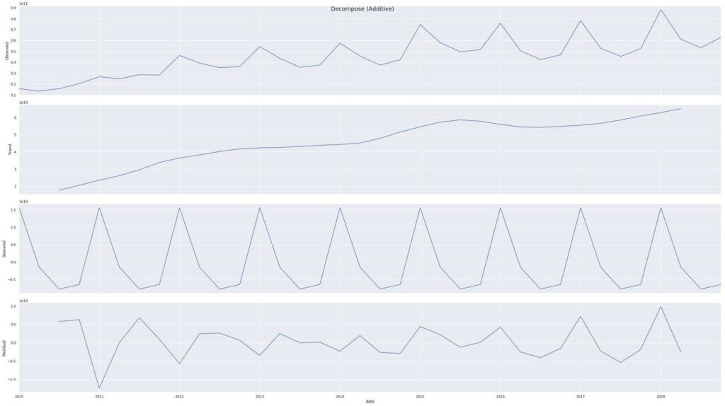
Again, we’re only trying to gain a conceptual understanding of each of these techniques.
Principal Component Analysis
Principal component analysis (PCA) reduces dataset dimensionality, increases interpretability, and minimizes information loss. It does so by creating new uncorrelated variables that successively maximize variance.
Said another way, data can often have many features, some important and some not. The idea is to distill the data down to the essential items and analyze from there.
Autoregression
Autoregression is a time series model that uses historical observations as input to a regression equation to predict the next step’s value. This is why it’s called autoregression — it “regresses against itself” as it uses data from the same input at previous time steps.
yt = b + c_1 * xt1 + c_2 * x_t2
Where b is the bias, c are coefficients, and x is the lagged time series steps.
Volatility Modeling
Volatility modeling attempts to forecast volatility to predict future returns. Often volatility models try to predict quantiles or absolute returns.
Stochastic volatility (SV) and GARCH are two well-known models used to predict financial time series volatility.
Statical Arbitrage Trading Strategies
Let’s walk through two market-neutral trading strategies.
If you’re familiar with Python and want to try your hand at creating a pair or triplet trading strategy, please see the Analyzing Alpha GitHub repo, demonstrating statistically significant mean reversion trading strategies.
This code is part of a series I created for Alpaca, an API-first brokerage.
Pairs Trading Strategy Walkthrough
We’ll now turn our gold and gold miner relationship into a pair trading strategy.
As discussed, pairs trading is a market-neutral strategy often implemented at hedge funds and investment banks attempting to profit from a stationary time series relationship.
Here are the steps we’ll follow:
- Find a cointegrating pair
- Create a synthetic asset
- Profit!
You’re sitting at your desk at the beginning of May 2007 and hypothesizing that gold and gold miners should be cointegrating. You would check TradingView, assuming it existed back then, to inspect the two stocks quickly.
You liked what you saw, so you tested for cointegration using a Cointegrated Augmented Dicky-Fuller (CADF) test in Python for the past year.
The CADF outputs that the two price series are cointegrating between 95-99% probability over that period and with the following formula:
SyntheticAsset = 1.0 _ GLD + -1.19 _ GDX
In other words, for every GLD you buy, you sell 1.19 GDX. A synthetic asset is just a fancy term for taking a long position and a short position in multiple securities simultaneously.
Instead of trading this every day, raking up transaction costs, you’re smart and decide to use Bollinger Bands and trade only when the synthetic asset gets “significantly” different from the norm.
You will take a short position when the market prices go above the top Bollinger band and establish a long position when the prices go below the Bollinger band. If a long or short touches the basis line at any time, you close your position by removing both from your portfolio.
So how did you do for the next year?
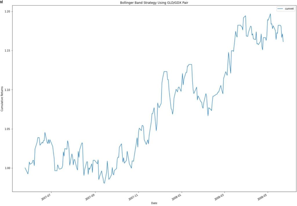
Nice job! You profited using a market-neutral pairs trading strategy more often used by hedge funds than retail traders.
You decide for the next pairs trade to use traditional technical analysis techniques and leverage to juice your returns even further while remembering that models can break at any time.
Triplets Trading Strategy Example
While a CADF test works for pairs trading, it does not work for triplet and multiple-asset arbitrage. For this, you’ll need the Johansen test.
The good news is that the only change you need to make is trading out the CADF function for the Johansen function.
There are also other mean reversion trading elements when exploiting an arbitrage opportunity, such as identifying how long it should take for a spread to revert to the mean. This is called the half-life of the mean, and for that, I highly recommend reading my favorite books on statistical arbitrage.
Statistical Arbitrage Books
If you’re interested in learning more about statistical arbitrage, I have two favorite books that I think are “significant’.