Timing the Markets with ETF Fund Flows

Due to poor investment timing, the average stock investor trails the market’s performance. The psychological forces of missing out (FOMO) are strong but lead to weak investment returns. An intelligent investor can utilize ETF fund flows to help time the market.

I’ve been busy lately, and it’s hard to believe it’s been almost two months since my last post. I decided to get something published today and thought it might be nice to explain some of the great pandas data manipulation seen in Our Own Worst Enemy by Chad Gray. I don’t want to take away from his readership; I’ll only be elaborating on the code and math to help less experienced algo traders and expect you to read his article to fill in the gaps where needed.

With this out of the way, let’s get started!

About Fund Flows

The critical understanding is that ETF fund flows create or destroy outstanding shares at the end of each day, depending upon inflow and outflows to the ETF. We can determine the behavioral gap by tracking the daily changes in outstanding shares compared to the price.

I’ll be using the ETF Fund Flows published by ETF Global. This data includes splits and dividends, so we won’t need to perform any adjustments.

Getting the ETF Price Data

First, let’s get the imports. I will be grabbing the ETF data from my local PSQL database. These are the imports starting with app. If you’re interested in doing the same, you can create your own PSQL database.

import matplotlib.pyplot as plt
import seaborn as sns
import numpy as np
import pandas as pd
from app.db.psql import db, session
from app.models.etf import EtfFundFlow, \
                           get_etf_fund_flows, \
                           get_sector_tickers

Next, create a function that adds the simple daily returns (R) and the daily log returns (r) to the get_etf_fund_flows dataframe.

def create_flow_data(tickers, start, end):
    ## Using convention for return identification:
    ## Simple returns denoted with capital R
    ## log returns identified by lowercase r
    etf_fund_flows = get_etf_fund_flows(tickers, start, end)
    etf_fund_flows['daily_R'] = etf_fund_flows['nav'].groupby(level='ticker').pct_change()
    etf_fund_flows['daily_r'] = np.log(etf_fund_flows['nav']).groupby(level=0).diff()
    etf_fund_flows['flow'] = np.log(etf_fund_flows['shares_outstanding']).groupby(level=0).diff()
    etf_fund_flows['mktcap'] = etf_fund_flows['nav'] * etf_fund_flows['shares_outstanding']
    etf_fund_flows.dropna(inplace=True)
    return etf_fund_flows

With the data in the format we need, let’s visualize the shares outstanding vs. price.

ticker = 'XLE'
xle = etf_fund_flows.loc[ticker]
xle['shares_outstanding'] \
       .plot(figsize=(16,10), legend=True)
xle['nav'].rename('price') \
       .plot(title=f"{ticker}: Shares Outstanding vs. Price",
             legend=True,
             secondary_y=True)
plt.show()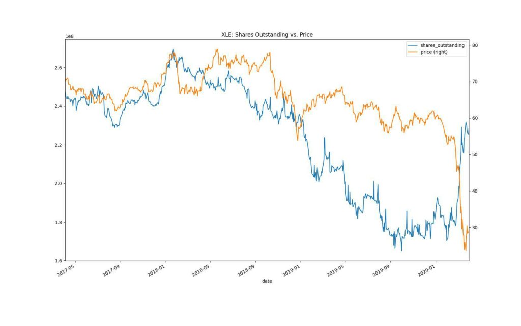

Notice how the nav, or the price, is separate from the shares outstanding.

Define the Return Formulae

We’ll start by creating a function that returns the simple annual return from an ETF fund flows dataframe. The function takes the mean of the daily log return, multiplies it by 252, which is the average number of trading days per year, “reverses” the log operation using np.exp and converts it to an annual percentage.

We convert them to log returns and then transform them back into simple returns. Imagine if we buy a stock for 1.00 that goes up 100% and then down 50%, our total geometric return would be 0%: 1.00 * (1+1) * (1+ -0.5) = $1.00.

Notice how the prior return affected the next? The arithmetic mean doesn’t consider this relationship and would be misleading, showing a 25% return: (1 + -0.5) / 2 = 25%. Log returns don’t have this limitation enabling us to add or multiply them, solving this issue.

def calc_etf_return(df):
    avg_daily_r = df['daily_r'].mean()
    annual_ret_log = avg_daily_r * 252
    annual_ret_simple = np.exp(annual_ret_log) - 1
    return annual_ret_simple * 100

Next up, we need to calculate the investor return.

We can determine how much the average investor is investing in any given ETF by looking at the daily changes in shares outstanding multiplied by the daily changes in the market cap. This assumes that we’re purchasing all of our shares at the new market cap value, but it gets us close enough. Let’s see this with an example.

Imagine on day zero we have 1.00 invested. If we double our shares outstanding, but the market cap drops by 50%, our new invested amount is 1 (day zero) + 1 * 1/2 (day one) = 1.50. Then on day two, we cut our shares in half with the market cap staying the same: 1.50 * 1/2 = 0.75. Now for each day, we know our amount invested. Make sense, right?

Now we can take the daily returns multiplied by the daily amount we have invested divided by the average amount invested. This gives us a return for each day. As shown below, we can then take the average of all of those returns and convert it back to a simple return.

def calc_investor_return(df):
    flows = df['flow'] * (df['mktcap'] / df['mktcap'].iloc[0])
    flows.iloc[0] = 1
    basis = flows.cumsum()

    avg_daily_r = (df['daily_r'] * basis / basis.mean()).mean()
    annual_ret_log = avg_daily_r * 252
    annual_ret_simple = np.exp(annual_ret_log) - 1
    return annual_ret_simple * 100

With both the ETF and investor return functions defined, let’s create a function to compare both annual returns for future graphing purposes.

First, we grab the tickers by getting the first level of the multiindex, passing it to unique, and then converting it to a list.

tickers = df.index.get_level_values(0).unique().tolist()

Next, we loop through each ticker, calculating the investor and investment return. We use .resample(‘A’) to group our dataframe into years (annual) and then apply our return functions. We then concatenate the data along with the index and return it. Default to concatenation before merge functions as it’s more performant.

If resampling and manipulating time data are new to you, please read Time Series Analysis with Python.

out = pd.DataFrame()
    for ticker in tickers:
        twr = df.loc[ticker].resample('A').apply(calc_etf_return)
        mwr = df.loc[ticker].resample('A').apply(calc_investor_return)
        twr.name = 'twr'
	mwr.name = 'mwr'
        both = pd.concat([twr, mwr], axis=1).reset_index()
        both['ticker'] = ticker
        both['timing_impact'] = both['mwr'] - both['twr']
        both.set_index(['date', 'ticker'], inplace=True)
        out = pd.concat([out, both], axis=0)
    return out

With the formulas defined, it’s now easy to analyze the results. Let’s create a list of tickers to explore the behavior gap. We’ll create a list of tickers and pass them to the functions we created earlier.

tickers = ['SPY', 'IWM', 'QQQ', 'VT']
flows = create_flow_data(tickers, start, end)

results = pd.DataFrame(columns=['investment', 'investor'])
for ticker in tickers:
   tmp = flows.xs(ticker, level='ticker', drop_level=True)
   print(tmp)
   results.loc[ticker, 'investment'] = calc_etf_return(tmp)
   results.loc[ticker, 'investor'] = calc_investor_return(tmp)
   results['behavioral_gap'] = results['investor'] - results['investment']
   print(results)

investment          investor      behavioral_gap
SPY    12.134     11.72          -0.414001
IWM    7.47855   7.15249     -0.326054
QQQ   19.0069   18.2117      -0.795162
VT       8.38496   7.82806      -0.556897

Interestingly, with updated data, investors consistently underperform the benchmark.

Let’s use some pandas magic to graph this.

by_year = compare_annual(flows)['timing_impact']
print(by_year)

date        ticker
2017-12-31  IWM       0.256712
2018-12-31  IWM       -1.601035
2019-12-31  IWM       1.562052
2017-12-31  QQQ      -0.132723
2018-12-31  QQQ      -1.543145
2019-12-31  QQQ      -0.639015
2017-12-31  SPY       -0.033773
2018-12-31  SPY       -0.310273
2019-12-31  SPY        0.025464
2017-12-31  VT          -0.120763
2018-12-31  VT          -0.811108
2019-12-31  VT          1.075920

Our multiindex contains both date and ticker. We can unstack this multiindex to convert the innermost index, which is the ticker, to columns. We’ll also round to two decimal places. Putting it all together:

by_year = compare_annual(flows)['timing_impact'].unstack().round(3)
print(by_year)

ticker        IWM    QQQ    SPY     VT
date
2017-12-31  0.257 -0.133 -0.034 -0.121
2018-12-31 -1.601 -1.543 -0.310 -0.811
2019-12-31  1.562 -0.639  0.025  1.076

We can then use Seaborn to create a heatmap to see the behavioral gap visually. We convert the index to just the year for graphing purposes.

by_year.index = by_year.index.year
sns.heatmap(by_year,
            center =0.00,
            cmap = sns.diverging_palette(10, 220, sep=1, n=21),
            annot=True)
plt.title('Behavioral Gap Heatmap')
plt.show()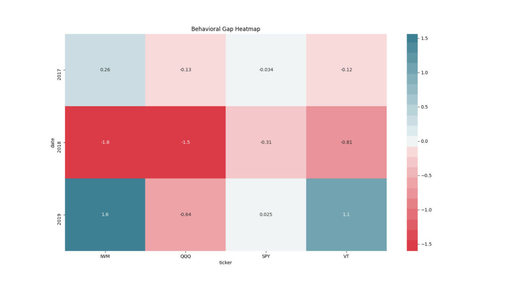

Hopefully, this post helps those on their way to becoming proficient with pandas and gives some of my readers a new potential contrarian signal to exploit.