If you’re interested in finance and don’t mind programming, learning this trio will open you up to a whole new world, including but not limited to, automated trading, backtest analysis, factor investing, portfolio optimization, and more.

I think of the Python, pandas, and NumPy combination as a more robust and flexible Microsoft Excel.

Python is extremely popular as it allows developers to create programs quickly without worrying about a lot of the details. It’s a high-level language. The problem with high-level languages is that they are often slow. The reason why Python is an excellent language for finance is that you get both the benefit of development speed with fast execution as both pandas and NumPy are highly optimized.

What is NumPy?

Let’s pretend we are calculating the price-to-earnings ratio for 800 stocks. We have two columns stored in lists with the first being price and the second being earnings. If we were to loop through each row, our CPU would need 800 cycles to convert the calculation into bytecode and then calculate the answer.

Vectorization

NumPy takes advantage of vectorization processing multiple calculations at a single time using Single Instruction Multiple Data (SIMD). While the loop may have taken 800 cycles, the vectorized computation may only take 200 cycles or even less.

NumPy also makes our life as a developer easier as it simplifies many of the everyday tasks we need to perform on a dataset. Take the below as an abbreviated example of the 800 stock scenario above:

Example Using Python and a List of Lists

price_earnings = [
                ['Company A', 10.0, 2.0],
                ['Company B', 30.0, 4.0],
                ['Company C', 50.0, 6.0],
                ['Company D', 70.0, 8.0],
                ['Company E', 90.0, 10.0]
                ]

pe_ratios = []

for row in price_earnings:
    pe_ratio = row[1] / row[2]
    pe_ratios.append(pe_ratio)

Example Using NumPy

pe_ratios = price_earnings[:,0] / price_earnings[:,1]

While you may not understand the exact syntax at the moment, you get the point: NumPy makes both development and execution faster. You can use any of the standard Python numeric operators in your vector math. The one catch, which is evident when you think about it, is that both vectors must be of the same shape and type such as a 5-item integer or 10-element float.

Creating a NumPy Array

import numpy as np
price_earnings = [
                ['Company A', 10.0, 2.0],
                ['Company B', 30.0, 4.0],
                ['Company C', 50.0, 6.0],
                ['Company D', 70.0, 8.0],
                ['Company E', 90.0, 10.0]
                ]

## Creating array from prior values
company_table = np.array(price_earnings)

## Autogenrate a 1D array
array1d = np.arange(10)

## Autogenerate a 2D array into 2 rows by 5 columns
array2d = array1d.reshape(2,5)

NumPy also makes it easy for us to calculate various statistics.

numpy.mean returns the average along the specified axis. numpy.ndarray.max returns the maximum value along a given axis. numpy.ndarray.min returns the minimum value along a given axis.

We’ve been discussing 1d or 1-dimensional arrays. You can think of these as equivalent to Excel columns.

2d or 2-dimensional arrays are like an Excel sheet where values are organized by both rows and columns. max, min, and mean will calculate the respective calculation across all of the cells of the 2d array unless we specify otherwise.

If we want to get the max of a row, we would specify ndarray.max(axis=1). If we want to find the max of each column, we would specify ndarray.max(axis=0) switching out the ndarray with your ndimensional array. When using these types of operations, all of the fields must be of the same type.

Selecting Data

Selecting data in NumPy is similar to highlighting and copying cells in Excel. The colon represents the entire row or column. When retrieving data from a NumPy 2D array, it uses the row, column format where both row and column can take a value or a list:

numpy_2d_array[row,column]

Common selection patterns

## Retrieve a single cell
cell = company_table[1,1]

## Retrieve the first row and all of the columns
row = company_table[0,:]

## Retreive all rows for the third column
column = company_table[:,2]

## Retreive two columns
two_columns = company_table[:,[0,2]]

## Retreive subsection
subsection = company_table[[0,2],[0,1]]

Selecting Data using Boolean Arrays

Sometimes called Boolean vectors or Boolean masks, Boolean arrays are an incredibly powerful tool. Booleans result in either True or False based upon a comparison operator such as greater than >, equal to == or less than <.

If we wanted to check for all stocks from the above example with a pe_ratio of less than 8, we could do the following:

low_pelow_pe_filter = pe_ratios < 8

This would return a 1D ndarray containing True and False values. I’ve added the other columns for readability, but again, the result would only be a single column:

Company	Price	Earnings	P/E Ratio	PE < 8
Company A	10	2	5.0	True
Company B	30	4	7.5	True
Company C	50	6	8.3	False
Company D	70	8	8.75	False
Company E	90	10	9.0	False

Once we have a Boolean mask, we apply it to the original array to filter the values we want. This is known as Boolean indexing.

low_pe_stocks = company_table[low_pe_filter]

Company	Price	Earnings	P/E Ratio
Company A	10	2	5.0
Company B	30	4	7.5

Working with a 2-dimensional mask is no different. We just have to make sure that the mask dimension is the same as the array dimension being filtered. See the below NumPy 2D array with working and incorrect examples.

2d_array = np.array([
                    [1,2,3,4],
                    [5,6,7,8],
                    [9,10,11,12],
                    [13,14,15,16],
                    [17,18,19,20]
                    ])

1	2	3	4
5	6	7	8
9	10	11	12
13	14	15	16
17	18	19	20

array2d = np.array([
                    [1,2,3,4],
                    [5,6,7,8],
                    [9,10,11,12],
                    [13,14,15,16],
                    [17,18,19,20]
                    ])

rows_mask = [True, False, False, True, True]
columns_mask = [True, True, False, True]

# working examples
works1 = array2d[rows_mask]
works2 = array2d[:, columns_mask]
works3 = array2d[rows_mask, columns_mask]

# incorrect examples due to dimension mismatch
does_not_work1 = array2d[columns_mask]
does_not_work2 = array2d[row_mask, row_mask]

Modifying Data

Now that we know how to select data, modifying data becomes easy. To modify the above array, we can simply assign a value to our selections.

# Change single value
array2d[0,0] = 5
array2d[0,0] = array2d[0,0] * 2

# Change row
array2d[0,:] = 0

# Change column
array2d[:,0] = 0

# Change a block
array2d[1:,[2,3]] = 0

# Change any value greater than 5 to 5
array2d[array2d > 5] = 5

# Change any value in column 2 greater than 5 to 5
array2d[array2d[:,1] > 5, 1] = 5

What Is Pandas?

Pandas is an extension of NumPy that builds on top of what we already know, supports vectorized operations, and makes data analysis and manipulation even easier.

Pandas has two core data types: Series and DataFrames.

A pandas Series is a one-dimensional object. It’s pandas version of the NumPy one-dimensional array.
A pandas DataFrame is a two-dimensional object. It’s similar to a NumPy 2D array.

Both pandas Series and pandas DataFrames are similar to their NumPy, equivalents but they both have additional features making manipulating data easier and more fun.

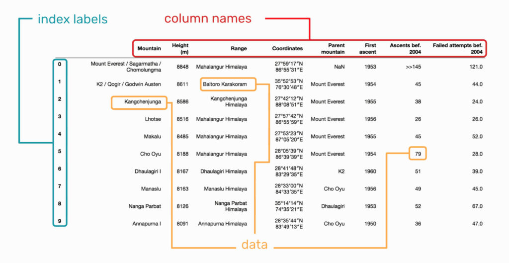
Both 2D NumPy arrays and Panda DataFrames have a row (index) and a column axis; however, the pandas versions can have named labels.

There are three main components of a DataFrame:

Index axis (row labels)
Columns axis (column labels)
Data (values)

See the below image sourced from Selecting data from a Pandas DataFrame

Creating a Pandas DataFrame

Generally, you’ll create a pandas dataframe by reading in records from a CSV, JSON, API, or database. We can also construct one from a dictionary as shown below.

dataframe.set_index allows you to change the index if desired.

data = {'company': ['Company A', 'Company B', 'Company C', 'Company D', 'Company E'],
        'price': [10, 30, 50, 70, 90],
        'earnings': [2.0, 4.0, 6.0, 8.0, 10.0]
        }

df = pd.DataFrame(data)

Creating a Pandas Series

Just like a dataframe, you’ll usually read in the data for a series from a CSV, JSON, API, or database. For example purposes, we’ll use the above dataframe to construct our series by returning a single column or row from our dataframe.

# Create a series
column_series = df['company']
row_series = df.loc[0]

The Data Types

Data is generally categorized as continuous or categorical. Continuous data is numeric and represents a measurement such as height, price or volume. Categorical data represents discrete amounts such as eye color, industry sector or share type.

Pandas data can be many different dtypes with the most common shown below:

General Type	Pandas String Name	NumPy / Pandas Object
Boolean	bool	np.bool
Integer	int	np.int
Float	float	np.float
Object	object	np.object
Datetime	datetime64	np.datetime64, pd.Timestamp
Timedelta	timedelta64	np.timedelta64, pd.Timedelta
Categorical	category	pd.Categorical

Understanding the Data

dataframe.info returns common information such as all of the dtypes, which is shorthand for datatypes, the shape, and other pertinent information regarding the dataframe. Notice that the order of the columns are not preserved.

df.info()

<class 'pandas.core.frame.DataFrame'>
RangeIndex: 5 entries, 0 to 4
Data columns (total 3 columns):
company     5 non-null object
earnings    5 non-null float64
price       5 non-null int64
dtypes: float64(1), int64(1), object(1)
memory usage: 192.0+ bytes

dataframe.index returns the row labels of the dataframe
dataframe.columns returns the column labels of the dataframe
dataframe.to_numpy returns the values of the dataframe
series.index returns the axis labels of the series
series.to_numpy returns the values of the series
series.dtype will return the type of the series, which again is just a single dimension of the dataframe.
dataframe.head returns 5 records starting at the top unless an int is passed.
dataframe.tail returns 5 records starting at the bottom unless an int is passed.
series.head returns int number of rows starting at the top.
series.tail returns int number of rows starting at the bottom.

print(df.head(2))
print(df.tail(2))

        company  earnings  price
0  Company A       2.0     10
1  Company B       4.0     30
        
        company  earnings  price
3  Company D       8.0     70
4  Company E      10.0     90

Selecting Data

We can select data in Pandas can be done with one of three indexers [], loc[] and iloc[]:

DataFrame[row_selection, column_selection] indexing operator best used for selecting columns.
DataFrame.loc[row_selection, column_selection] index rows and columns by labels inclusive of the last column
DataFrame.iloc[row_selection, column_selection] index rows and columns by integer exclusive of the last integer postion
Series.loc[index_selection] index rows by the index label.
Series.iloc[index_selection] index rows by the integer position.

Shortcuts for Selecting Data

The shortcut dataframe[‘label’] can be used when selecting a single row or list of rows. The shortcut dataframe[‘label1′:’label3′] can be used for slicing rows; however, I believe using dataframe.loc and dataframe.iloc when performing row selection as it makes what you’re doing more explicit.

## Retrieve a single cell
cell = df.loc[1,'price']

## Retrieve the first row and all of the columns
row = df.loc[0,:]

## Retreive all rows for the third column
column = df.loc[:,'earnings']
column_short = df['earnings']

## Retreive a range of rows
rows = df.loc[1:3]
rows_short = df[1:3]

## Retreive two columns
two_columns = df.loc[:,['company','earnings']]
two_columns_by_position = df.iloc[:,[0,2]]
two_columns_short = df[['company','earnings']]

## Retrieve a range of columns
range_of_columns = df.loc[:,'earnings':'price']
range_of_columns_by_position = df.iloc[:,1:3]

## Retreive subsection
subsection = df.loc[0:2,['company','price']]

## Selecting from Series
## Selecting a single cell
cell = column_series.loc[1]
cell_short = column_series[1]

## Selecting a range of cells from a column
cell_range = column_series.loc[0:3]
cell_range_short = column_series[0:3]

## Selecting a range of cells from a row
cell_range = row_series.loc['company':'price']
cell_range_short = row_series['company':'price']

Understanding Data

Pandas dataframes and series are both unique objects so they have different methods; however, many methods are implemented for both dataframes and series as shown below. Large numbers are shown in E-notation.

Series.describe and DataFrame.describe returns descriptive statistics. We can use method chaining to return a pandas series and then describe it as shown in the second example below. Describe works differently on numeric and non-numeric values.

print(df.describe())

            price   earnings
count   5.000000   5.000000
mean   50.000000   6.000000
std    31.622777   3.162278
min    10.000000   2.000000
25%    30.000000   4.000000
50%    50.000000   6.000000
75%    70.000000   8.000000
max    90.000000  10.000000

print(df['price'].describe())
count     5.000000
mean     50.000000
std      31.622777
min      10.000000
25%      30.000000
50%      50.000000
75%      70.000000
max      90.000000
Name: price, dtype: float64

print(df['company'].describe())
count             5
unique            5
top       Company B
freq              1
Name: company, dtype: object

For some dataframe methods we’ll need to specify if we want to calculate the result across the index or columns. For example, if we sum across the row values (index), we’ll get a result for each column. If we sum across all of the column values, we’ll get a result for each row.

To remember the axis numbers, I remember how to reference a dataframe[0,1] where 0 is the first position and represents rows and 1 is our second position and represents columns. And while 0 represents calculating down rows, it’s also often the default and doesn’t need to be explicitly stated. If you’re still having trouble remembering the order, you can think that a 0 will add another row and a 1 will add another column.

Series.sum and DataFrame.sum returns the sum for the requested axis.
Series.mean and DataFrame.mean returns the mean of the requested axis.
Series.median and DataFrame.median returns the median for the requested axis.
Series.mode and DataFrame.mode returns the mode for the requested axis.
Series.max and DataFrame.max returns the maximum value for the requested axis.
Series.min and DataFrame.min returns the minimum value for the requested axis.
Series.count and DataFrame count return the number of non-NA elements.
Series.value_counts returns the unique value counts as a series.

## Sum across columns
df[['earnings','price']].sum(axis=1)

## Sum across rows
## Sum across rows calculating a value for each column. This is the default
df[['earnings','price']].sum()
df[['earnings','price']].sum(axis=0)

Standard Operations Between Two Series

As with NumPy, we can utilize all of the Python numeric operations on two panda series returning the resultant series.

## Standard Operation examples
print(df[['earnings','price']] + 10)
    earnings  price
0      12.0     20
1      14.0     40
2      16.0     60
3      18.0     80
4      20.0    100

df['pe_ratio'] = df['price'] / df['earnings']
print(df)
        company  price  earnings  pe_ratio
0  Company A     10       2.0  5.000000
1  Company B     30       4.0  7.500000
2  Company C     50       6.0  8.333333
3  Company D     70       8.0  8.750000
4  Company E     90      10.0  9.000000

Assigning Values

Now that we understand selection, assignment becomes trivial. It’s just like NumPy only we can use the pandas selection shortcuts. This includes both assignment and assignment using Boolean indexing. See the examples below from the dataframe selection section. Note that I set the index to company instead of using a numeric index.

# Assignment
df.set_index('company', inplace=True)
#df.loc['Company B', 'pe_ratio'] = 0.0

## Assignment to a single element
df.loc['Company B','price'] = 0.0

## Assignment to an entire row
df.loc['Company B',:] = 0

## Assignment to an entire column
df.loc[:,'earnings'] = 0.0
df['earnings'] = 1.0

## Assignment to a range of rows
df.loc['Company A':'Company C'] = 0.0
df['Company A':'Company C'] = 1.0

## Assignment to two columns
df.loc[:,['price','earnings']] = 2.0
df[['price','earnings']] = 3.0

## Assignment to a range of columns
df.loc[:,'earnings':'pe_ratio'] = 4.0

## Assignment to a subsection
df.loc['Company A':'Company C',['price','earnings']] = 5.0

## Assignment using boolean indexing
### Using boolean value
price_bool = df['price'] < 4.0
df.loc[price_bool,'price'] = 6.0

### Skipping boolean value
df.loc[df['price'] >= 4, 'price'] = 7.0

What is NumPy?

Vectorization

Selecting Data

Common selection patterns

Selecting Data using Boolean Arrays

Modifying Data

What Is Pandas?

Creating a Pandas DataFrame

Creating a Pandas Series

The Data Types

Understanding the Data

Selecting Data

Shortcuts for Selecting Data

Understanding Data

Standard Operations Between Two Series

Assigning Values

Leave a Comment Cancel reply

Share this Article

Python for Finance: An Easy Introduction

What is NumPy?

Vectorization

Selecting Data

Common selection patterns

Selecting Data using Boolean Arrays

Modifying Data

What Is Pandas?

Creating a Pandas DataFrame

Creating a Pandas Series

The Data Types

Understanding the Data

Selecting Data

Shortcuts for Selecting Data

Understanding Data

Standard Operations Between Two Series

Assigning Values

Leave a Comment Cancel reply

Subscribe to the Newsletter

Share this Article