What Is Stationarity? A Visual Guide

Stationarity means that a process’s statistical properties that create a time series are constant over time. This statistical consistency makes distributions predictable enabling forecasting, and is an assumption of many time series forecasting models.

What Is Stationarity?

In mathematics and statistics, a stationary process is a stochastic process whose unconditional joint probability distribution does not change when shifted in time. Said more simply, we can slice up the time series data into equally sized chunks for a stationary time series and still get the same probability distribution.

There are multiple types of stationarity, which we’ll cover below. But for now, let’s understand the general concept of stationarity through visual exploration.

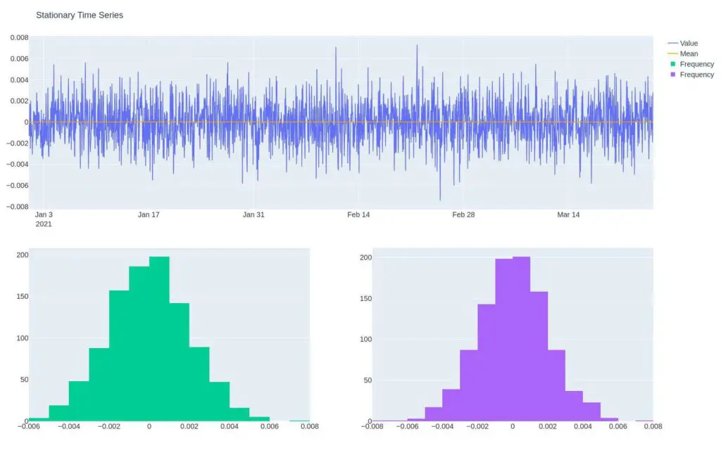
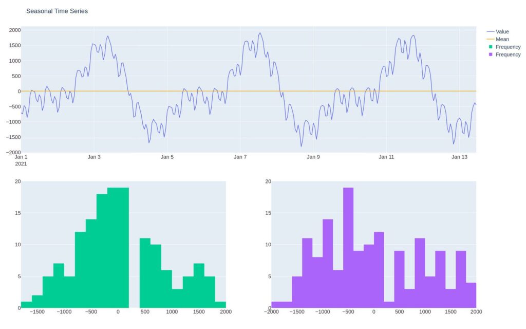
Notice the line chart and histogram below. The line chart shows multiple values oscillating around a mean of zero. The histogram, in green, displays the frequency of values in the shape of a normal distribution.

Why Is Stationarity Important?

A stationary process, another way to say something that generates a stationary time series, has specific statistical properties enabling predicting a likely outcome.

For instance, in the histogram above, we can see the most likely value is near zero, and as we move away from zero, the values we get are less likely.

As algorithmic traders, we can build a mean reversion trading system to profit from a stationary time series. If the price is stretched too far from its normal distribution, we expect it to revert to the mean.

Most time series in the markets are not stationary. We can attempt to convert a non-stationary stochastic process to a stationary one using methods such as differencing, or we can create a synthetic asset that combines multiple holdings to make a stationary process.

A stochastic process is one where the process has some randomness. It’s the opposite of a deterministic process where the outcome has 100% certainty.

Fun fact: Stochastic derives from stokhazesthai, the Greek word to guess or aim.

Now that we know what a stationary process is, let’s solidify our understanding by looking at a few non-stationary stochastic processes.

Non-Stationary Stochastic Processes

As I mentioned earlier, a non-stationary process is a stochastic process that doesn’t have a consistent mean or distribution across time. This typically comes in the form of trend, volatility, or seasonality.

Let’s explore visually and with code.

Trend

Notice the time series below doesn’t have a consistent mean, and its distribution changes through time, making it difficult to predict the next value in its current form.

But each value is just a cumulative sum of the prior values, so there is a predictable trend—more on this in the types of stationarity section.

df2 = pd.DataFrame(index=dti,data=np.random.random(size=periods) * vol).cumsum()
make_plot(df2, "Trending Time Series").show()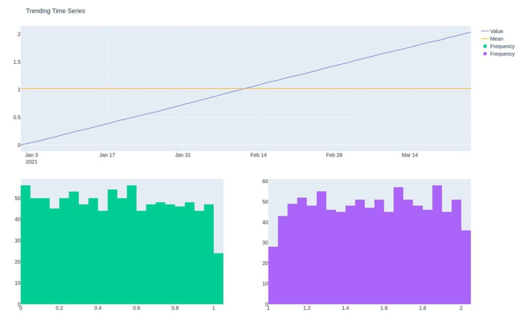

Variance

The below time series has a consistent mean, but its volatility increases. The increase in variance changes the distribution of values through time. Notice while the mean in the distribution is the same, the values are more extreme in the second half of the time series.

df3 = pd.DataFrame(index=dti,
    data=np.random.normal(size=periods) * vol *
        np.logspace(1,5,num=periods, dtype=int))
make_plot(df3, "Volatility Increasing Time Series").show()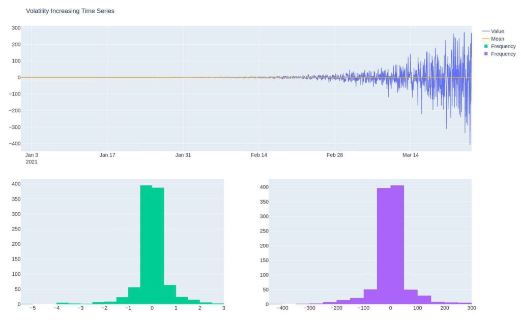

Seasonality

Seasonality refers to a series whose distribution changes predictably through time. An example of this would be Google trends search interest for beach and ski resorts.

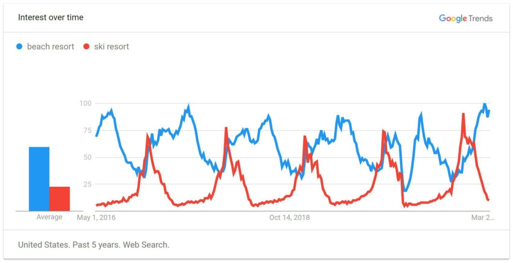
We can see that interest in the beach is highest when it’s warm, and ski-goers search for resorts when it’s cold. Both follow a predictable, seasonal pattern. We can compare each quarter with last year’s quarter to make things more predictable. Speaking of predictable…

Seasonality is different from cyclicality. Seasonality is predictable, whereas cyclicality is not.

Skipping the code on this one as it’s more complex, and I feel like it doesn’t aid in understanding seasonality.

If interested, check it out on the Analyzing Alpha GitHub Repo.

Notice that the distribution changes through time.

This is obvious. If we look at the revenue of a ski resort in the winter months, it’ll be vastly different from its revenue when the sun’s shining.

Noise

White noise is a time series with a mean of zero, its volatility is constant, and there’s no correlation between lags — its variables are independent and identically distributed variables.

In other words, it’s random.

If it’s not random, we can create a better forecasting model by extracting the non-random signal from the random noise.

We can decompose our time series into components: Signal – the time series data we can potentially predict noise – the part of the data set that’s unpredictable

y(t) = signal_t + noise_t

If we can prove that our residuals (signal minus noise) are white noise, we can say our model is great.

df4 = pd.DataFrame(index=dti,
                   data=np.random.normal(size=periods) * vol)
make_plot(df4, "White Noise").show()

Types of Stationarity

There are multiple types of stationarity. Understanding moments is vital to grasping the various types of stationarity. The goal of this section isn’t to be exhaustive; it’s to give you a basic intuitive understanding of each type of stationarity.

Strong Stationarity

So far, we’ve been discussing strong stationarity. Strong stationarity means that the random value produced has the same probability distribution across time for any event.

Weak Stationarity

Weak stationarity, also known as wide-sense stationarity, has a constant mean (moment one) and the correlation and covariance (moment two) are invariant to time. The higher-order moments change with time.

N-th Order Stationarity

N-th order stationarity means that the process generating the time series has a moment invariant to time.

• First-order stationarity – Constant mean.
• Second-order stationarity – Constant variance and is first-order stationarity.
• Third-order stationarity – Constant skew and is second-order stationarity
• Forth-order stationary – Constant kurtosis and is third-order stationarity

Trend Stationarity

Trend stationarity means removing the trend from an underlying stochastic process, creating a stationary process.

Recall the trending time series above. The time series is just a normally distributed random value plus all previous values. We can subtract the earlier values from each point to make the time series stationary. In other words, the process is trend stationarity.

Joint Stationarity

Most processes in the markets are not stationary. One way to create stationary processes, as mentioned above, is to combine multiple stochastic processes that cointegrate.

We can use this cointegrating pair to create a synthetic asset in a pairs-trading strategy.

The Bottom Line

Stationarity refers to a random process that has constant statistical properties through time. This matters because it means that the process creates a predictable distribution. Stationarity is a common assumption for many time series models.