Traders using technical analysis attempt to profit from supply and demand imbalances. Technicians use price and volume patterns to identify these potential imbalances to profit from them. Algorithmic chart pattern detection allows traders to scan more charts while eliminating bias.
In this post, I will review how to detect chart patterns algorithmically and create a quick backtest in Backtrader. This work expands on posts found on Alpaca and Quantopian analyzing the paper:
Before we get started, you’ll want to grab data. If you do not have a data provider, you can grab a free Intrinio developer sandbox.
Get The Data
import pandas as pd
from positions.securities import get_security_data
aapl = get_security_data('AAPL', start='2020-03-01', end='2020-03-31')
print(aapl)
open high low close volume
date
2020-03-02 282.280 301.4400 277.72 298.81 85349339
2020-03-03 303.670 304.0000 285.80 289.32 79868852
2020-03-04 296.440 303.4000 293.13 302.74 54794568
2020-03-05 295.520 299.5500 291.41 292.92 46893219
2020-03-06 282.000 290.8200 281.23 289.03 56544246
2020-03-09 263.750 278.0900 263.00 266.17 71686208
2020-03-10 277.140 286.4400 269.37 285.34 71322520
2020-03-11 277.390 281.2200 271.86 275.43 64094970
2020-03-12 255.940 270.0000 248.00 248.23 104618517
2020-03-13 264.890 279.9200 252.95 277.97 92683032
2020-03-16 241.950 259.0800 240.00 242.21 80605865
2020-03-17 247.510 257.6100 238.40 252.86 81013965
2020-03-18 239.770 250.0000 237.12 246.67 75058406
2020-03-19 247.385 252.8400 242.61 244.78 67964255
2020-03-20 247.180 251.8300 228.00 229.24 100423346
2020-03-23 228.080 228.4997 212.61 224.37 84188208
2020-03-24 236.360 247.6900 234.30 246.88 71882773
2020-03-25 250.750 258.2500 244.30 245.52 75900510
2020-03-26 246.520 258.6800 246.36 258.44 63140169
2020-03-27 252.750 255.8700 247.05 247.74 51054153
2020-03-30 250.740 255.5200 249.40 254.81 41994110
2020-03-31 255.600 262.4900 252.00 254.29 49250501Find the Minama and Maxima
Chart patterns can be determined from local minima and maxima. From a technical analysis perspective, this is really just the highs and the lows.
We can find the price highs and lows using scipy.signal.argregexterma.
argrelextrema takes in an ndarray and a comparable and returns a tuple with an array of the results. The comparables we’ll use will be np.greater and np.less. Here’s a simple example for demonstration purposes:
from scipy.signal import argrelextrema
x = np.array([2, 1, 2, 3, 2, 0, 1, 0])
argrelextrema(x, np.greater)
(array([3, 6]),)Notice how the 4th and 6th elements are the relative highs — remember arrays start with zero. The same goes for our lows.
from scipy.signal import argrelextrema
x = np.array([2, 1, 2, 3, 2, 0, 1, 0])
argrelextrema(x, np.less)
(array([1, 5]),)With an understanding of how to calculate our highs and lows, let’s do the same with Apple’s price data. We’ll grab the first element of the tuple returned by argrelextrema.
local_max = argrelextrema(aapl['high'].values, np.greater)[0]
local_min = argrelextrema(aapl['low'].values, np.less)[0]
print(local_max)
print(local_min)
This gives us the index position of the relative highs and lows. Let’s verify this.
[ 1  6  9 13 18]
[ 5  8 12 15]
We can index Apple’s rows by integer. We’ll then check out TradingView to see if our results match up.
highs = aapl.iloc[local_max,:]
lows = aapl.iloc[local_min,:]

print(highs)
print(lows)
date
2020-03-03 304.00
2020-03-10 286.44
2020-03-13 279.92
2020-03-19 252.84
2020-03-26 258.68
Name: high, dtype: float64
date
2020-03-09 263.00
2020-03-12 248.00
2020-03-18 237.12
2020-03-23 212.61
Name: low, dtype: float64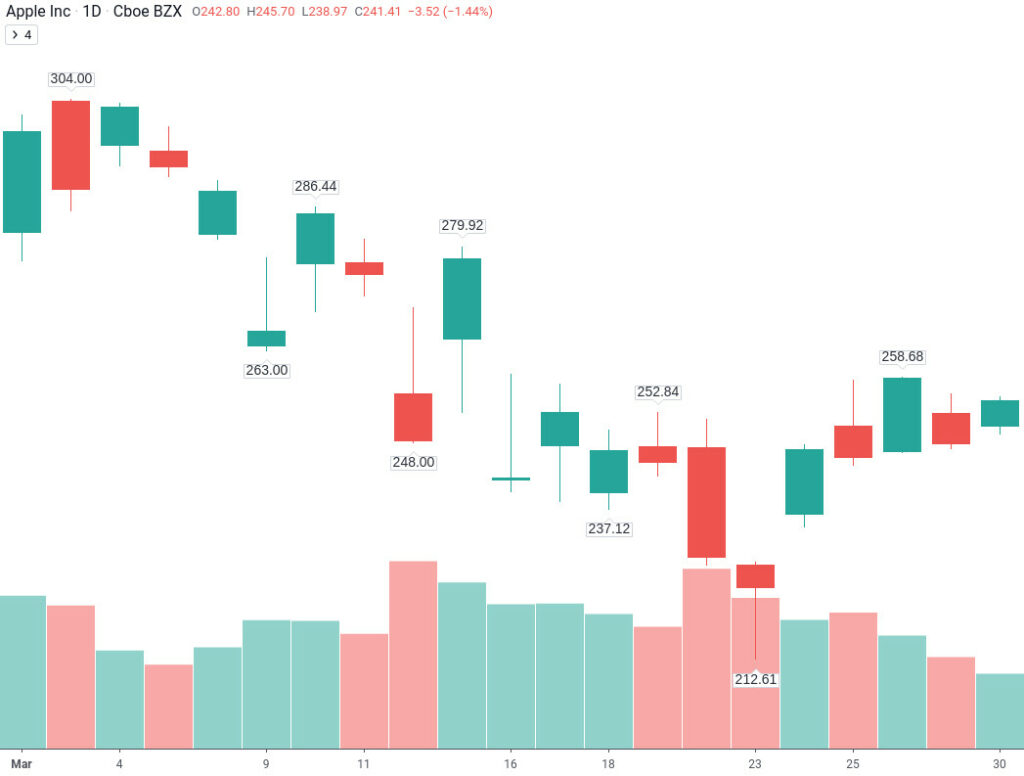
While not as pretty, we can also graph it in Matplotlib.
import matplotlib.pyplot as plt
fig = plt.figure(figsize=[20,14])
highslows = pd.concat([highs,lows])
aapl['high'].plot()
aapl['low'].plot()
plt.scatter(highslows.index,highslows)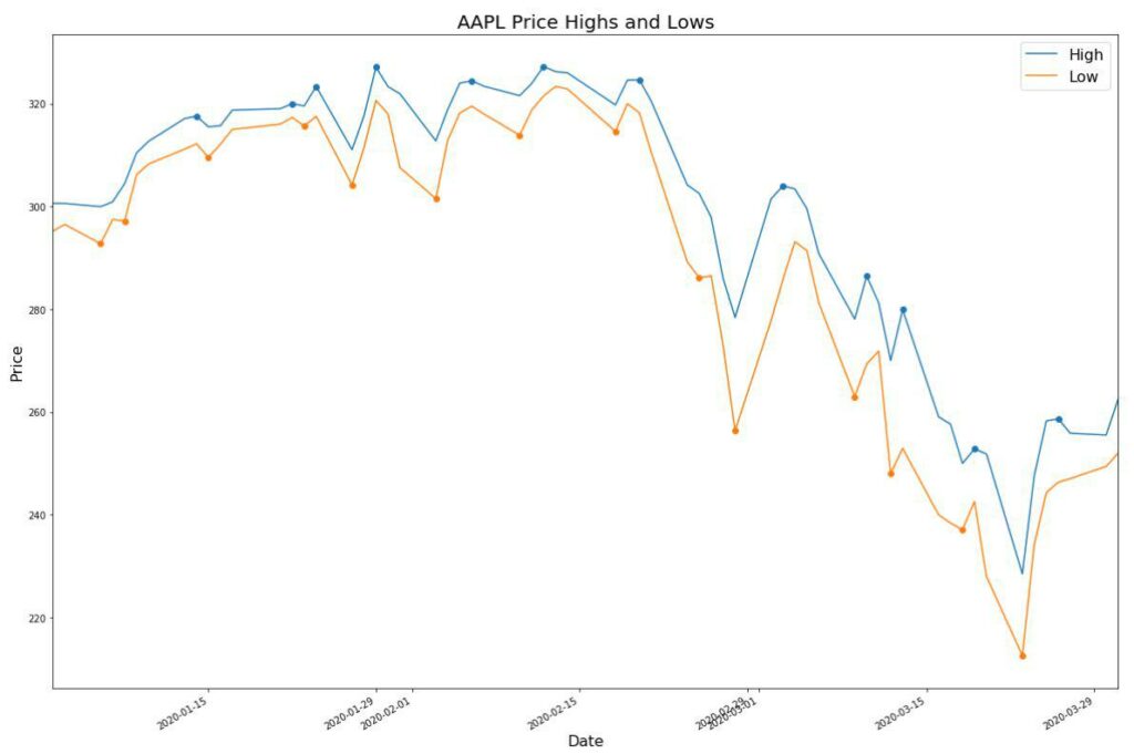
We can use the local minima and maxima to determine trend changes. We’ll use the paper’s notation when discussing extrema.
Where E_t is a local extrema with price P_t, therefore, we can now determine uptrends and downtrends based on local extrema. An uptrend consists of higher highs and higher lows. A downtrend consists of lower highs and lower lows. Here are the formulas for an uptrend and a downtrend, respectively.
Uptrend: E_1 < E_3 and E_2 < E_4
Downtrend: E_1 > E_3 and E_2 > E_4
Smoothing the Noise
In the paper, Andrew Lo uses smoothing and non-parametric kernel regression with the idea of reducing the noise in the price action. Don’t worry, we’ll dig into what non-parametric kernel regression is in a minute. For now, let’s smooth out Apple’s prices. We’ll use pandas.series.rolling for this purpose using a window of 2.
fig = plt.figure(figsize=[20,14])
aapl['close'].plot()
aapl['close'].rolling(window=5).mean().plot()
Notice how the graph becomes smoother even though we lose some data.
Non-Parametric Kernel Regression
Let’s analyze this statistical term word by word:
- Nonparametric means the data does not fit a normal distribution. We know this. Stock price prediction is complex.
- In nonparametric statistics, a kernel is a weighting function.
- Regression predicts the value of the predictor based on information in the data.
Non-parametric kernel regression is another way to smooth our prices. The idea is that we approximate a price average based on prices near the predicted price using a weighting the closest prices more heavily.
So what does this look like with code?
from statsmodels.nonparametric.kernel_regression import KernelReg
kr = KernelReg(prices_.values, prices_.index, var_type='c')
f = kr.fit([prices_.index.values])
aapl['close'].rolling(window=4).mean().plot()
smooth_prices = pd.Series(data=f[0], index=aapl.index)
smooth_prices.plot()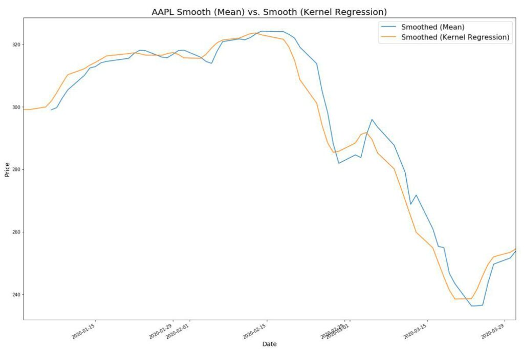
Notice how we don’t lose data. We can also adjust the bandwidth to change the fit.
from statsmodels.nonparametric.kernel_regression import KernelReg
kr = KernelReg(prices_.values, prices_.index, var_type='c', bw=[1])
kr2 = KernelReg(prices_.values, prices_.index, var_type='c', bw=[3])
f = kr.fit([prices_.index.values])
f2 = kr2.fit([prices_.index.values])

smooth_prices = pd.Series(data=f[0], index=aapl.index)
smooth_prices2 = pd.Series(data=f2[0], index=aapl.index)
smooth_prices.plot()
smooth_prices2.plot()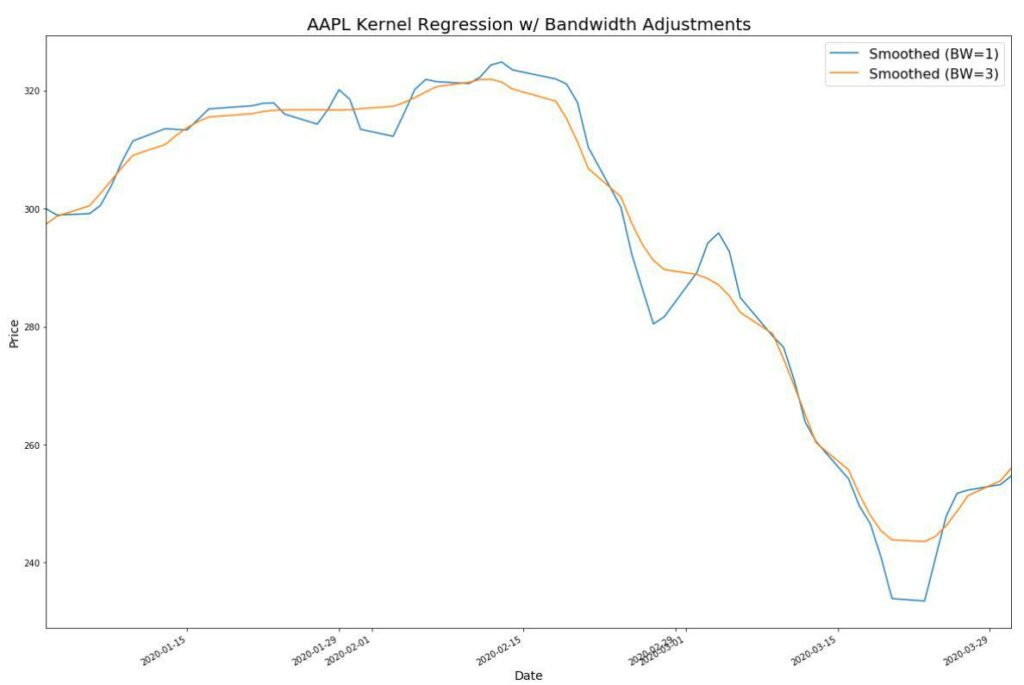
Let’s find our local maxima and minima using the smoothed prices using kernel regression with a bandwidth of 0.85.
kr = KernelReg(prices_.values, prices_.index, var_type='c', bw=[0.85])
f = kr.fit([prices_.index.values])
smooth_prices = pd.Series(data=f[0], index=aapl.index)
smoothed_local_maxima = argrelextrema(smooth_prices.values, np.greater)[0]
print(smoothed_local_maxima)
print(local_maxima)
[ 2 6 18]
[ 1 6 9 13 18]Notice that we now skip over local minima, which may be considered noise.
With our smoothed prices, let’s loop through the extrema and grab the highest value in a two-day window before and after our extrema.
price_local_max_dt = []
for i in smoothed_local_max:
    if (i>1) and (i<len(aapl)-1):
        price_local_max_dt.append(aapl['close'].iloc[i-2:i+2].idxmax())

price_local_min_dt = []
for i in smoothed_local_min:
    if (i>1) and (i<len(aapl)-1):
        price_local_min_dt.append(aapl['close'].iloc[i-2:i+2].idxmin())


max_min = pd.concat([aapl.loc[price_local_min_dt, 'close'], aapl.loc[price_local_max_dt, 'close']])
aapl['close'].plot()
plt.scatter(max_min.index, max_min.values, color='orange')
Let’s put everything we’ve done so far into a function.
from scipy.signal import argrelextrema
from statsmodels.nonparametric.kernel_regression import KernelReg

def find_extrema(s, bw='cv_ls'):
    """
    Input:
        s: prices as pd.series
        bw: bandwith as str or array like
    Returns:
        prices: with 0-based index as pd.series
        extrema: extrema of prices as pd.series
        smoothed_prices: smoothed prices using kernel regression as pd.series
        smoothed_extrema: extrema of smoothed_prices as pd.series
    """
    # Copy series so we can replace index and perform non-parametric
    # kernel regression.
    prices = s.copy()
    prices = prices.reset_index()
    prices.columns = ['date', 'price']
    prices = prices['price']

    kr = KernelReg([prices.values], [prices.index.to_numpy()], var_type='c', bw=bw)
    f = kr.fit([prices.index])

    # Use smoothed prices to determine local minima and maxima
    smooth_prices = pd.Series(data=f[0], index=prices.index)
    smooth_local_max = argrelextrema(smooth_prices.values, np.greater)[0]
    smooth_local_min = argrelextrema(smooth_prices.values, np.less)[0]
    local_max_min = np.sort(np.concatenate([smooth_local_max, smooth_local_min]))
    smooth_extrema = smooth_prices.loc[local_max_min]

    # Iterate over extrema arrays returning datetime of passed
    # prices array. Uses idxmax and idxmin to window for local extrema.
    price_local_max_dt = []
    for i in smooth_local_max:
        if (i>1) and (i<len(prices)-1):
            price_local_max_dt.append(prices.iloc[i-2:i+2].idxmax())

    price_local_min_dt = []
    for i in smooth_local_min:
        if (i>1) and (i<len(prices)-1):
            price_local_min_dt.append(prices.iloc[i-2:i+2].idxmin())

    maxima = pd.Series(prices.loc[price_local_max_dt])
    minima = pd.Series(prices.loc[price_local_min_dt])
    extrema = pd.concat([maxima, minima]).sort_index()

    # Return series for each with bar as index
    return extrema, prices, smooth_extrema, smooth_prices
Let’s use Matplotlib to visualize the output.
def plot_window(prices, extrema, smooth_prices, smooth_extrema, ax=None):
    if ax is None:
        fig = plt.figure()
        ax = fig.add_subplot(111)

    prices.plot(ax=ax, color='dodgerblue')
    ax.scatter(extrema.index, extrema.values, color='red')
    smooth_prices.plot(ax=ax, color='lightgrey')
    ax.scatter(smooth_extrema.index, smooth_extrema.values, color='lightgrey')

plot_window(prices, extrema, smooth_prices, smooth_extrema)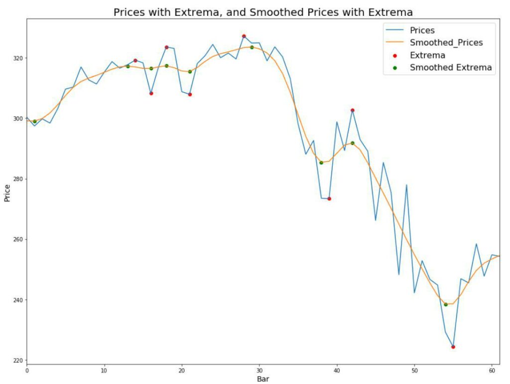
Pattern Identification
I will use the pattern definitions from the paper. The code is largely taken from the Quantopian post mentioned earlier, with a few adjustments to fit my needs.
from collections import defaultdict

def find_patterns(s, max_bars=35):
    """
    Input:
        s: extrema as pd.series with bar number as index
        max_bars: max bars for pattern to play out
    Returns:
        patterns: patterns as a defaultdict list of tuples
        containing the start and end bar of the pattern
    """
    patterns = defaultdict(list)

    # Need to start at five extrema for pattern generation
    for i in range(5, len(extrema)):
        window = extrema.iloc[i-5:i]

        # A pattern must play out within max_bars (default 35)
        if (window.index[-1] - window.index[0]) > max_bars:
            continue

        # Using the notation from the paper to avoid mistakes
        e1 = window.iloc[0]
        e2 = window.iloc[1]
        e3 = window.iloc[2]
        e4 = window.iloc[3]
        e5 = window.iloc[4]

        rtop_g1 = np.mean([e1,e3,e5])
        rtop_g2 = np.mean([e2,e4])
        # Head and Shoulders
        if (e1 > e2) and (e3 > e1) and (e3 > e5) and \
            (abs(e1 - e5) <= 0.03*np.mean([e1,e5])) and \
            (abs(e2 - e4) <= 0.03*np.mean([e1,e5])):
                patterns['HS'].append((window.index[0], window.index[-1]))

        # Inverse Head and Shoulders
        elif (e1 < e2) and (e3 < e1) and (e3 < e5) and \
            (abs(e1 - e5) <= 0.03*np.mean([e1,e5])) and \
            (abs(e2 - e4) <= 0.03*np.mean([e1,e5])):
                patterns['IHS'].append((window.index[0], window.index[-1]))

        # Broadening Top
        elif (e1 > e2) and (e1 < e3) and (e3 < e5) and (e2 > e4):
            patterns['BTOP'].append((window.index[0], window.index[-1]))

        # Broadening Bottom
        elif (e1 < e2) and (e1 > e3) and (e3 > e5) and (e2 < e4):
            patterns['BBOT'].append((window.index[0], window.index[-1]))

        # Triangle Top
        elif (e1 > e2) and (e1 > e3) and (e3 > e5) and (e2 < e4):
            patterns['TTOP'].append((window.index[0], window.index[-1]))

        # Triangle Bottom
        elif (e1 < e2) and (e1 < e3) and (e3 < e5) and (e2 > e4):
            patterns['TBOT'].append((window.index[0], window.index[-1]))

        # Rectangle Top
        elif (e1 > e2) and (abs(e1-rtop_g1)/rtop_g1 < 0.0075) and \
            (abs(e3-rtop_g1)/rtop_g1 < 0.0075) and (abs(e5-rtop_g1)/rtop_g1 < 0.0075) and \
            (abs(e2-rtop_g2)/rtop_g2 < 0.0075) and (abs(e4-rtop_g2)/rtop_g2 < 0.0075) and \
            (min(e1, e3, e5) > max(e2, e4)):

            patterns['RTOP'].append((window.index[0], window.index[-1]))

        # Rectangle Bottom
        elif (e1 < e2) and (abs(e1-rtop_g1)/rtop_g1 < 0.0075) and \
            (abs(e3-rtop_g1)/rtop_g1 < 0.0075) and (abs(e5-rtop_g1)/rtop_g1 < 0.0075) and \
            (abs(e2-rtop_g2)/rtop_g2 < 0.0075) and (abs(e4-rtop_g2)/rtop_g2 < 0.0075) and \
            (max(e1, e3, e5) > min(e2, e4)):
            patterns['RBOT'].append((window.index[0], window.index[-1]))

    return patterns
patterns = find_patterns(extrema)
print(patterns)
It looks like Apple’s prices contained both a broadening top and bottom. While having a small amount of data made things easier to see at first, let’s up the ante and detect the patterns within ten years of Google price data. I increased the non-parametric kernel regression bandwidth to 1.5.
googl = get_security_data('GOOGL', start='2019-01-01', end='2020-01-31')
prices, extrema, smooth_prices, smooth_extrema = find_extrema(googl['close'], bw=[1.5])
patterns = find_patterns(extrema)

for name, pattern_periods in patterns.items():
    print(f"{name}: {len(pattern_periods)} occurences")
HS: 2 occurences
TBOT: 3 occurences
TTOP: 1 occurences
RTOP: 1 occurences
BBOT: 1 occurences
BTOP: 1 occurencesLet’s graph the head and shoulder patterns.
for name, pattern_periods in patterns.items():
    if name=='HS':
        print(name)

        rows = int(np.ceil(len(pattern_periods)/2))
        f, axes = plt.subplots(rows,2, figsize=(20,5*rows))
        axes = axes.flatten()
        i = 0
        for start, end in pattern_periods:
            s = prices.index[start-1]
            e = prices.index[end+1]

            plot_window(prices[s:e], extrema.loc[s:e],
                        smooth_prices[s:e],
                        smooth_extrema.loc[s:e], ax=axes[i])
            i+=1
        plt.show()
Head & Shoulders Patterns
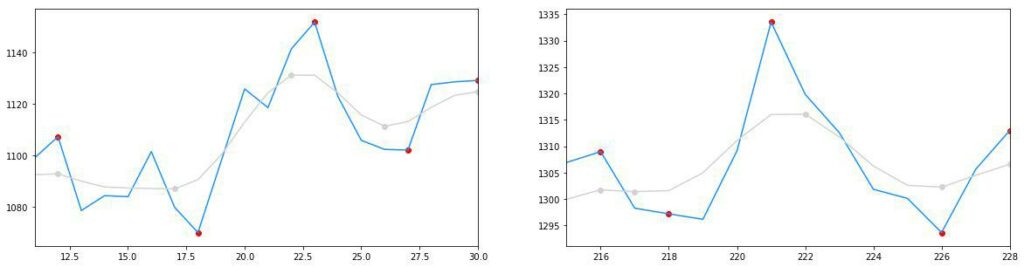
These do indeed look like head and shoulder patterns. Remember, the far-right edge will have the top of the shoulder. Additionally, if you’re not happy with the pattern definitions, you can change them!
While I’ve already created a Backtrader Backtesting Quickstart, I thought it might be nice to demonstrate how to take some of the above code and turn it into an indicator.
import pandas as pd
import numpy as np
import backtrader as bt
from scipy.signal import argrelextrema
from positions.securities import get_security_data


class Extrema(bt.Indicator):
    '''
    Find local price extrema. Also known as highs and lows.

        Formula:
        - https://docs.scipy.org/doc/scipy/reference/generated/scipy.signal.argrelextrema.html

        See also:
        - /algorithmic-pattern-detection

        Aliases: None
        Inputs: high, low
        Outputs: he, le
        Params:
        - period N/A
    '''
    lines = 'lmax',  'lmin'

    def next(self):

        # Get all days using ago with length of self
        past_highs = np.array(self.data.high.get(ago=0, size=len(self)))
        past_lows = np.array(self.data.low.get(ago=0, size=len(self)))

        # Use argrelextrema to find local maxima and minima
        last_high_days = argrelextrema(past_highs, np.greater)[0] \
            if past_highs.size > 0 else None
        last_low_days = argrelextrema(past_lows, np.less)[0] \
            if past_lows.size > 0 else None

        # Get the day of the most recent local maxima and minima
        last_high_day = last_high_days[-1] \
            if last_high_days.size > 0 else None
        last_low_day = last_low_days[-1] \
            if last_low_days.size > 0 else None

        # Use local maxima and minima to get prices
        last_high_price = past_highs[last_high_day] \
            if last_high_day else None
        last_low_price = past_lows[last_low_day] \
            if last_low_day else None

        # If local maxima have been found, assign them
        if last_high_price:
            self.l.lmax[0] = last_high_price

        if last_low_price:
            self.l.lmin[0] = last_low_price
Chart Pattern Backtest Results
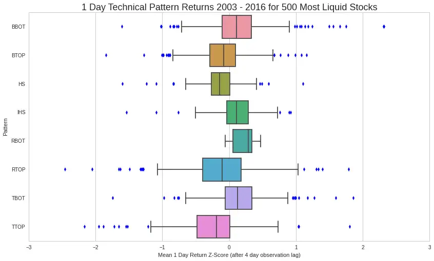
The Bottom Line
It does appear that certain technical patterns have predictive power. We can use code to detect these patterns and exploit them on multiple timeframes. As always, the code can be found on GitHub.