You can use visual inspection, global vs. local analysis, and statistics to analyze stationarity. The Augmented Dickey-Fuller (ADF) test is the most commonly used parametric test, and the Zivot-Andrews test is better than the ADF at detecting stationarity through structural breaks.
This post assumes you understand what stationarity is and why it’s important.
Note: I use matplotlib plots for analysis and Plotly charts for presentation in this post. The complete code for this post is on the Analyzing Alpha GitHub Repository.
Visual Inspection
It’s easy to see if a process is creating a stationary time series. If we see the mean or the distribution changing, it’s non-stationary.
Let’s first create a random walk model using Python, and then we’ll plot it in Plotly.
# Grab imports
import numpy as np
import pandas as pd

# Create index
periods = 2000
vol = .002
dti = pd.date_range("2021-01-01",
                    periods=periods,
                    freq="H")

# Generate normal distribution
random_walk = pd.DataFrame(index=dti,
                   data=np.random.normal(size=periods)  * vol)

# Plot it using a custom function
make_plot(random_walk,
          "Stationary "Random Walk" Time Series").show()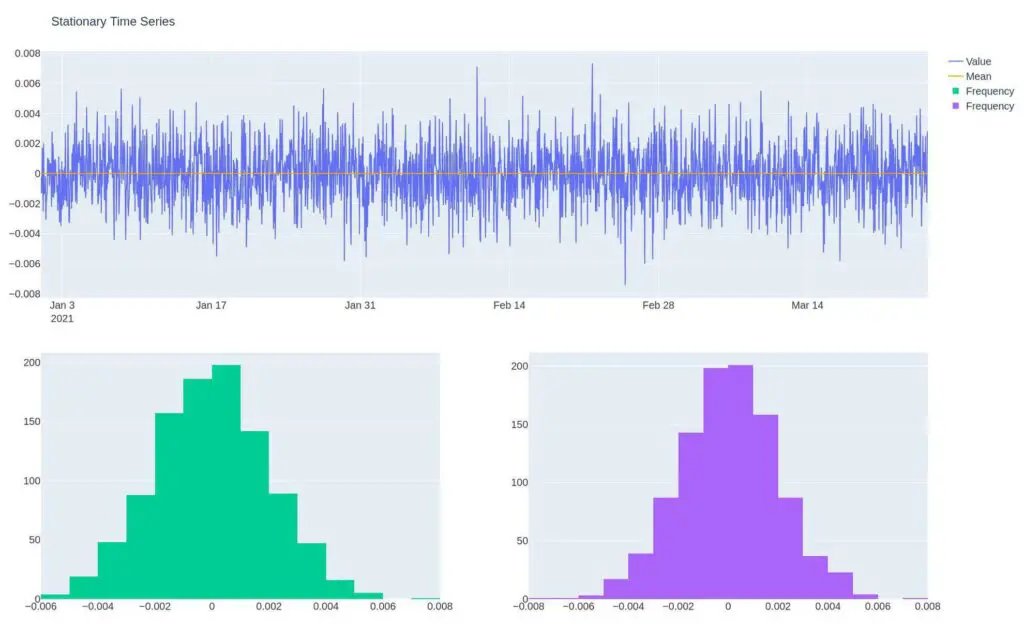
We can identify a stochastic process by analyzing a time series plot and gain an understanding of if there’s a shift in the mean or distribution through time. This is called global vs. local analysis, which we’ll discuss further below.
However, in practice, it’s trivial to use more advanced plot functions to identify a stationary process.
Decomposition
Time series decomposition separates the signal, trend, seasonality, and error automatically. Let’s decompose Apple’s revenue. We can see the clear seasonality and trend in this non-stationary data.
from statsmodels.tsa.seasonal import seasonal_decompose
sd = seasonal_decompose(apple_revenue_history)
sd.plot()
Autocorrelation Function
The autocorrelation and partial-autocorrelation functions analyze a data set for statistical significance between the first data point and prior data points.
A non-stationary time series data will show significance between itself and its lagged values, and that significance will decay to zero slowly as in the first plot.
The second plot, a stationary time series, will quickly drop to zero. The red lines are confidence intervals where values above or below the lines are more significant than two standard deviations.
from statsmodels.graphics.tsaplots import plot_acf
plot_acf(df2, lags=40, alpha=0.05)
plot_acf(df2.diff().dropna(), lags=40, alpha=0.05)
Sometimes it’s evident after visual inspection that we have stationary or non-stationary data. But even in these circumstances, we want to test our hypothesis using statistical tests to understand our series better.
Global vs. Local Analysis
We can break our time series into multiple segments and analyze the summary statistics of each against the time series or another partition to see if our time series data is changing through time.
def get_quads(df):
    quadlen = int(len(df1) * 0.25)
    ss = df[:quadlen].describe()
    ss[1] = df[quadlen:quadlen*2].describe()
    ss[2] = df[quadlen*2:quadlen*3].describe()
    ss[3] = df[quadlen*3:].describe()
    return ss
Random Walk
Notice how the random walk time series has a constant mean, variance, and the distribution between the min, percentages, and max are relatively consistent (no seasonality)?
random_walk = pd.DataFrame(index=dti,
                   data=np.random.random(size=periods) * vol)
get_quads(random_walk)
0 1 2 3
count 500.000000 500.000000 500.000000 500.000000
mean 0.000136 -0.000054 0.000070 -0.000216
std 0.002067 0.001909 0.002008 0.002020
min -0.005851 -0.005614 -0.006003 -0.006325
25% -0.001263 -0.001344 -0.001262 -0.001492
50% 0.000095 -0.000094 0.000045 -0.000229
75% 0.001503 0.001225 0.001331 0.001073
max 0.007002 0.006702 0.006338 0.005969Trend Stationary
You can see the mean is increasing in the trending time series.
trending = pd.DataFrame(index=dti,
                   data=np.random.random(size=periods) * vol).cumsum()
get_quads(trending)
0 1 2 3
count 500.000000 500.000000 500.000000 500.000000
mean 0.253949 0.754164 1.245338 1.752112
std 0.148433 0.138083 0.153263 0.144376
min 0.001630 0.509963 0.989912 1.509835
25% 0.122746 0.637347 1.111457 1.629752
50% 0.261204 0.749095 1.243160 1.748031
75% 0.376252 0.878295 1.376870 1.879781
max 0.508350 0.989398 1.509197 2.000878Volatile Time Series
The standard deviation is changing in the volatile time series.
varying = pd.DataFrame(index=dti,
                   data=np.random.normal(size=periods) * vol \
              * np.logspace(1,5,num=periods, dtype=int))
0 1 2 3
count 500.000000 500.000000 500.000000 500.000000
mean 0.000510 0.082075 -0.206946 -1.990338
std 0.094116 0.935861 10.263379 99.674838
min -0.664262 -3.887168 -46.277549 -472.434713
25% -0.039151 -0.280147 -4.025722 -45.672561
50% -0.001081 0.067228 -0.068825 -4.059768
75% 0.037203 0.476481 3.295115 35.828933
max 0.424776 5.000719 61.889090 455.791059Seasonal Time Series
You can identify seasonality by analyzing the distribution through min, max, and the percentages in between. Notice how the 50% area is changing.
def simulate_seasonal_term(periodicity, total_cycles, noise_std=1.,
                           harmonics=None):
    duration = periodicity * total_cycles
    assert duration == int(duration)
    duration = int(duration)
    harmonics = harmonics if harmonics else int(np.floor(periodicity / 2))

    lambda_p = 2 * np.pi / float(periodicity)

    gamma_jt = noise_std * np.random.randn((harmonics))
    gamma_star_jt = noise_std * np.random.randn((harmonics))

    total_timesteps = 100 * duration # Pad for burn in
    series = np.zeros(total_timesteps)
    for t in range(total_timesteps):
        gamma_jtp1 = np.zeros_like(gamma_jt)
        gamma_star_jtp1 = np.zeros_like(gamma_star_jt)
        for j in range(1, harmonics + 1):
            cos_j = np.cos(lambda_p * j)
            sin_j = np.sin(lambda_p * j)
            gamma_jtp1[j - 1] = (gamma_jt[j - 1] * cos_j
                                 + gamma_star_jt[j - 1] * sin_j
                                 + noise_std * np.random.randn())
            gamma_star_jtp1[j - 1] = (- gamma_jt[j - 1] * sin_j
                                      + gamma_star_jt[j - 1] * cos_j
                                      + noise_std * np.random.randn())
        series[t] = np.sum(gamma_jtp1)
        gamma_jt = gamma_jtp1
        gamma_star_jt = gamma_star_jtp1
    wanted_series = series[-duration:] # Discard burn in

    return wanted_series

duration = 100 * 3
periodicities = [10, 100]
num_harmonics = [3, 2]
std = np.array([2, 3])
np.random.seed(8678309)

terms = []
for ix, _ in enumerate(periodicities):
    s = simulate_seasonal_term(
        periodicities[ix],
        duration / periodicities[ix],
        harmonics=num_harmonics[ix],
        noise_std=std[ix])
    terms.append(s)
terms.append(np.ones_like(terms[0]) * 10.)
seasonal = pd.DataFrame(index=dti[:duration],data=np.sum(terms, axis=0))
                0            1            2            3
count    75.000000    75.000000    75.000000    75.000000
mean    328.055459  -280.450561  -149.840302   120.579444
std     733.650363   750.299351   958.572453  1007.596395
min    -863.464617 -1694.424423 -1815.786373 -1733.291362
25%    -239.600008  -770.199418  -828.906000  -694.550888
50%      72.425299  -346.127307  -405.201792    59.358360
75%     923.255524    59.875525   485.926284   945.035545
max    1813.015082  1642.090923  1916.794045  1832.084148
Parametric Tests
Statistical tests identify specific types of stationarity. Most parametric tests analyze if the time series has a unit root, which is a systematic pattern that is random in the presence of serial correlation — which is a fancy way of saying a lagged version of itself. The reason it’s called a unit root test is due to the math of the process.
Testing if the time series has a unit root and is therefore not stationary is the null hypothesis, which is a fancy way of saying the commonly accepted belief. We want to reject the null hypothesis with a level of certainty to state the time series is stationary — or more accurately, the process generating the time series is stationary.
Let’s look at the most common unit root tests.
Dickey-Fuller
The Dickey-Fuller test is the first statistical test that analyzes if a unit root exists in an autoregressive model of a time series.
It runs into issues with serial correlation, which is why there’s an Augmented Dickey-Fuller test.
Augmented Dickey-Fuller (ADF)
The Augmented Dickey-Fuller tests for a unit root in a univariate process in the presence of serial correlation. The ADF test handles more complex models and is the typical go-to for most analysts.
Non-Stationary Process
Let’s use the ADF test on Apple’s revenue, which is non-stationary.
from statsmodels.tsa.stattools import adfuller
t_stat, p_value, _, _, critical_values, _  = adfuller(df6['observed'].values, autolag='AIC')
print(f'ADF Statistic: {t_stat:.2f}')
for key, value in critical_values.items():
     print('Critial Values:')
     print(f'   {key}, {value:.2f}')
ADF Test Statistic: -2.12
Critial Values:
1%, -3.69
Critial Values:
5%, -2.97
Critial Values:
10%, -2.63You can compare the ADF test statistic of -2.12 against the critical values. We see that the test statistic is less than all of the critical values, so we cannot reject the null hypothesis — in other words, as we already knew, Apple’s revenue is non-stationary; we see trends, and it’s mean and variance are changing.
Stationary Process
Now let’s do the same for the random walk data, which exhibits stationarity.
from statsmodels.tsa.stattools import adfuller
result = adfuller(random_walk[0].values, autolag='AIC')
t_stat, p_value, _, _, critical_values, _  = adfuller(random_walk[0].values, autolag='AIC')
print(f'ADF Statistic: {t_stat:.2f}')
for key, value in critical_values.items():
     print('Critial Values:')
     print(f'   {key}, {value:.2f}')

print(f'\np-value: {p_value:.2f}')
print("Non-Stationary") if p_value > 0.05 else print("Stationary")
ADF Statistic: -43.83
Critial Values:
1%, -3.43
Critial Values:
5%, -2.86
Critial Values:
10%, -2.57
p-value: 0.00
StationaryNotice that this time I’ve included the p-value. When a p-value is greater than 5%, we accept the null hypothesis. We also see an extreme ADF test statistic from this random walk model.
I like the critical value approach compared to the p-value as I can see to what degree I can reject that the time series is not stationary.
Kwiakowski-Phillips-Schmidt-Shin (KPSS)
The Kwiatkowski-Phillips-Schmidt-Shin (KPSS) tests for the null hypothesis that the time series process is stationary or trend stationarity. In other words, the KPSS test null hypothesis is the opposite of the ADF test.
Exhibits Non-Stationarity
from statsmodels.tsa.stattools import kpss
t_stat, p_value, _, critical_values = kpss(df6['observed'].values, nlags='auto')

print(f'ADF Statistic: {t_stat:.2f}')
for key, value in critical_values.items():
     print('Critial Values:')
     print(f'   {key}, {value:.2f}')

print(f'\np-value: {p_value:.2f}')
print("Stationary") if p_value > 0.05 else print("Non-Stationary")
ADF Statistic: 0.91
Critial Values:
   10%, 0.35
Critial Values:
   5%, 0.46
Critial Values:
   2.5%, 0.57
Critial Values:
   1%, 0.74

p-value: 0.01
Non-Stationary
Exhibits Stationarity
from statsmodels.tsa.stattools import kpss
t_stat, p_value, _, critical_values = kpss(random_walk[0].values, nlags='auto')

print(f'ADF Statistic: {t_stat:.2f}')
for key, value in critical_values.items():
     print('Critial Values:')
     print(f'   {key}, {value:.2f}')

print(f'\np-value: {p_value:.2f}')
print("Stationary") if p_value > 0.05 else print("Non-Stationary")
from statsmodels.tsa.stattools import kpss
t_stat, p_value, _, critical_values = kpss(random_walk[0].values, nlags='auto')
print(f'ADF Statistic: {t_stat:.2f}')
for key, value in critical_values.items():
print('Critial Values:')
print(f' {key}, {value:.2f}')
print(f'\np-value: {p_value:.2f}')
print("Non-Stationary") if p_value > 0.05 else print("Stationary")Zivot and Andrews
Zivot-Andrews tests for the same thing as the ADF and KPSS tests for the presence of a structural break.
Let’s add a break to our random walk model. Notice how the variance and cyclicality properties are relatively constant, but there’s a significant shift in the mean.

Now let’s run both an ADF test and a Zivot-Andrews to test for non-stationarity.
t_stat, p_value, _, _, critical_values, _  = adfuller(stationary_with_break[0].values, autolag='AIC')
print(f'ADF Statistic: {t_stat:.2f}')
for key, value in critical_values.items():
     print('Critial Values:')
     print(f'   {key}, {value:.2f}')

print(f'\np-value: {p_value:.2f}')
print("Non-Stationary") if p_value > 0.05 else print("Stationary")
ADF Statistic: -1.05
Critial Values:
1%, -3.43
Critial Values:
5%, -2.86
Critial Values:
10%, -2.57
p-value: 0.73
Non-Stationaryfrom statsmodels.tsa.stattools import zivot_andrews
t_stat, p_value, critical_values, _, _ = zivot_andrews(stationary_with_break[0].values)
print(f'Zivot-Andrews Statistic: {t_stat:.2f}')
for key, value in critical_values.items():
print('Critial Values:')
print(f' {key}, {value:.2f}')
print(f'\np-value: {p_value:.2f}')
print("Non-Stationary") if p_value > 0.05 else print("Stationary")Zivot-Andrews Statistic: -60.35
Critial Values:
1%, -5.28
Critial Values:
5%, -4.81
Critial Values:
10%, -4.57
p-value: 0.00
StationaryWe see different results between the two stationarity tests. The ADF test fails to incorporate the structural break while the Zivot-Andrew identifies the series as stationary.
The Bottom Line
The process for testing for stationarity in time series data is relatively straightforward. You analyze the information visually, perform a decomposition, review the summary statistics, and then select a parametric test to gain confidence in your assumptions.
The Augmented Dickey-Fuller or ADF test is the most commonly used test for stationarity; however, it’s not always the best. To analyze stationarity in time series with structural breaks, you’ll want to use the Zivot-Andrews test. As always, it’s essential to have an intuitive understanding of the problem set and to have a deep knowledge of the tools at your disposal.