How to Make a Time Series Stationary in Python

You can make a time series stationary using adjustments and transformations. Adjustments such as removing inflation simplify the historical data making the series more consistent. Transforms like logarithms can stabilize the variance, while differencing transforms stabilize the mean from trend and seasonality.

You’ll learn the most popular methods to achieve stationarity in this post. You’ll also turn the price of Bitcoin into a stationary series for future predictive modeling.

You should already understand what stationarity is and how to determine if a time series is stationary.

The code for this post is at the Analyzing Alpha GitHub Repository.

Stationarity

Time series data is different than cross-sectional data. Time series are sets of data observed at successive points in time. In other words, order matters. With cross-sectional data, time is of no significance.

The temporal nature of time series data makes it uniquely challenging to model. Because order matters and most time series forecasting models assume stationarity, we must make non-stationary data stationary.

In particular, we need to remove the trend, variance, and seasonal components. Let’s analyze the price of Bitcoin and plot it to see if it’s stationary, and if it’s not (it isn’t), we’ll attempt to make it a stationary series.

import urllib
import pandas as pd
import zipfile

repo = 'https://raw.githubusercontent.com/leosmigel/analyzingalpha/master/'
file = 'time-series-analysis-with-python/btc_price_history.zip'
url = repo + file

with urllib.request.urlopen(url) as f:
  btc_price_history = pd.read_csv(f, compression='gzip',
                                  parse_dates=['btc_price_history.csv'])
  btc_price_history = btc_price_history.rename(
      columns={'btc_price_history.csv':'date'}
  )
  btc_price_history.set_index('date', inplace=True)
btc_price_history.dropna(inplace=True)

make_plot(btc_price_history['close'], "Bitcoin Price History").show()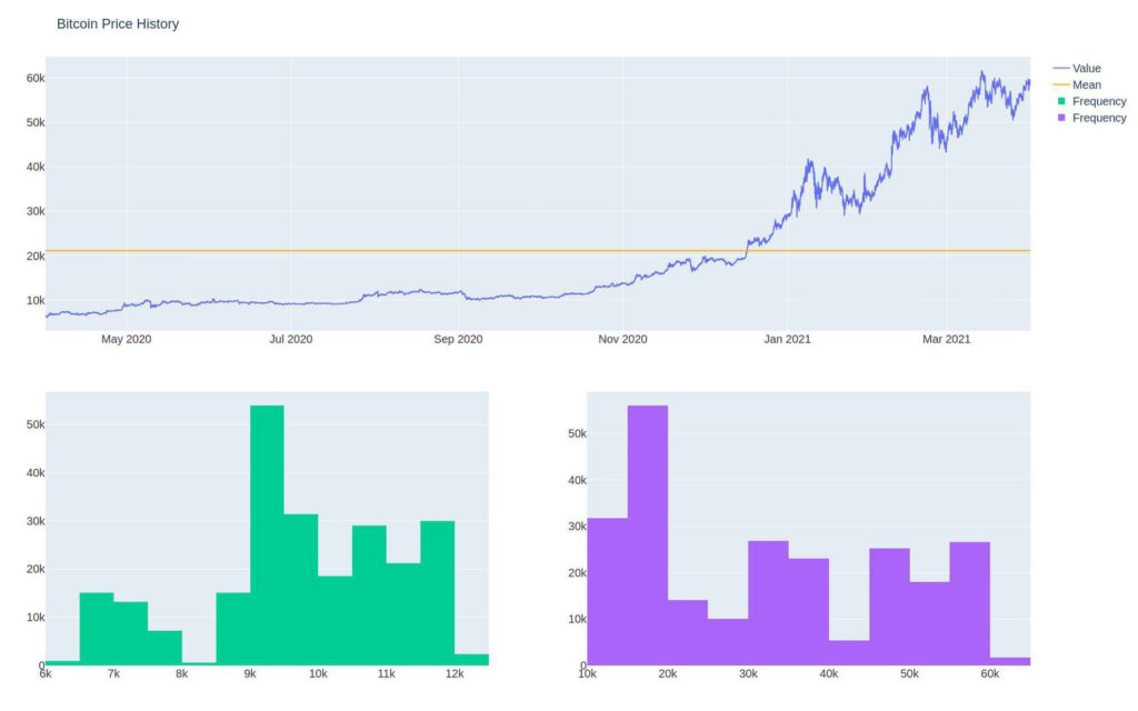

We can easily see that the price of Bitcoin is not stationary. A clear trend exists, and the variance is increasing.

Adjustments

Adjustments make historical data more simple or remove known patterns. Typically, fall into the following categories:

• Calendar Adjustments
• Population Adjustments
• Composition Adjustments

Calendar Adjustments

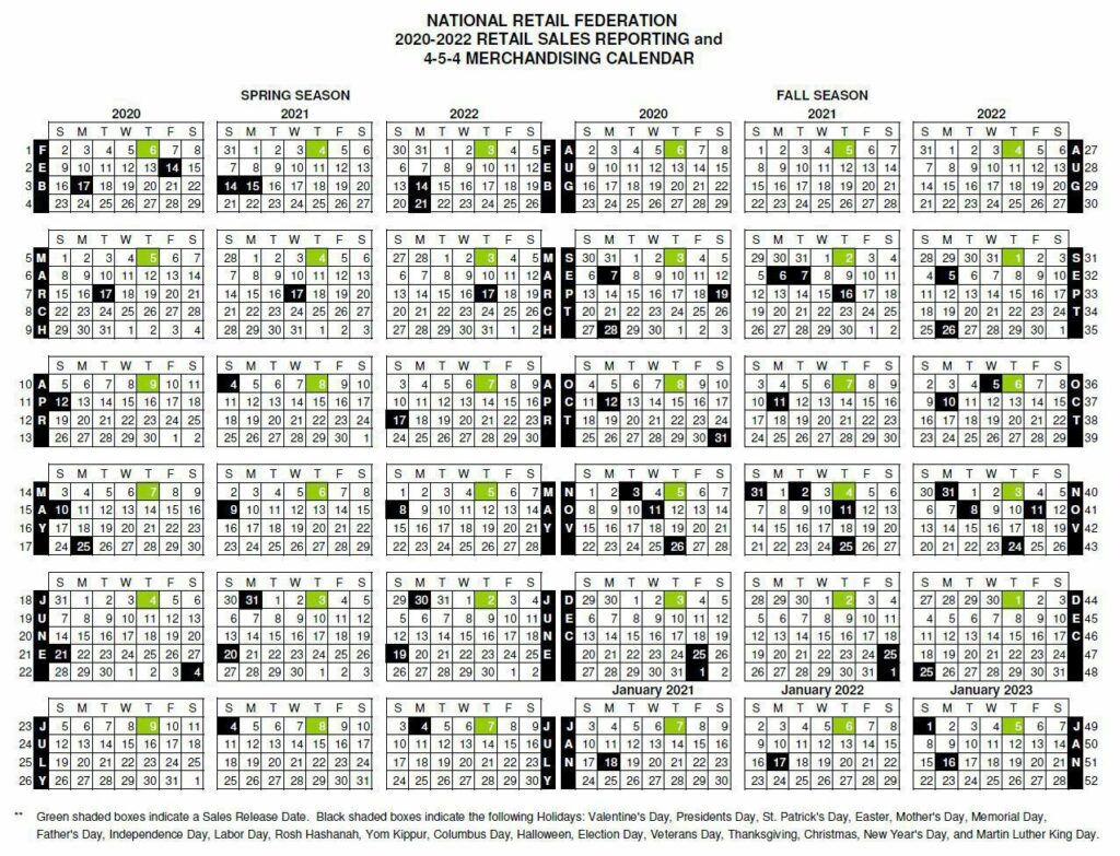
Calendar adjustments are pretty standard, especially when it comes to tracking sales. Businesses want to have comparability between months and years. If one month has 31 days and another has 28, it’s not exactly a fair comparison. Adjusting the monthly data ensures a fair comparison. This is precisely why most retailers follow a 4-5-4 calendar.

454 Retail Calendar

Population Adjustments

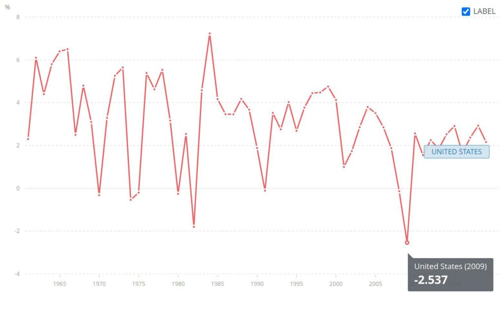
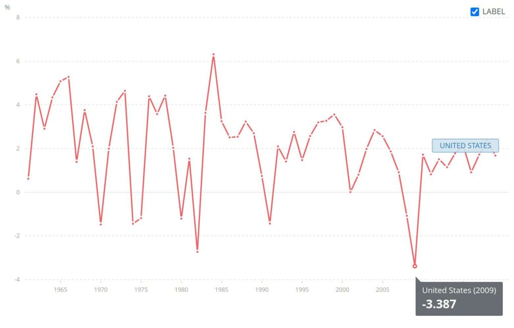
Population adjustments remove the effects of increasing or decreasing populations from the sample. The most common way to do this is to adjust the data per capita, which is just a ratio of the data over some proportion of the population — such as for every 1000.

See the GDP growth vs. GDP growth per capita from World Bank. There’s a substantial difference between the two — especially when analyzed on a percentage basis.

GDP Growth

Composition Adjustments

Composition adjustments remove or normalize component(s) from the analyzed time series. Having a good contextual understanding of the time series components is critical.

For instance, it’s essential to adjust for inflation when analyzing financial time series over long periods.

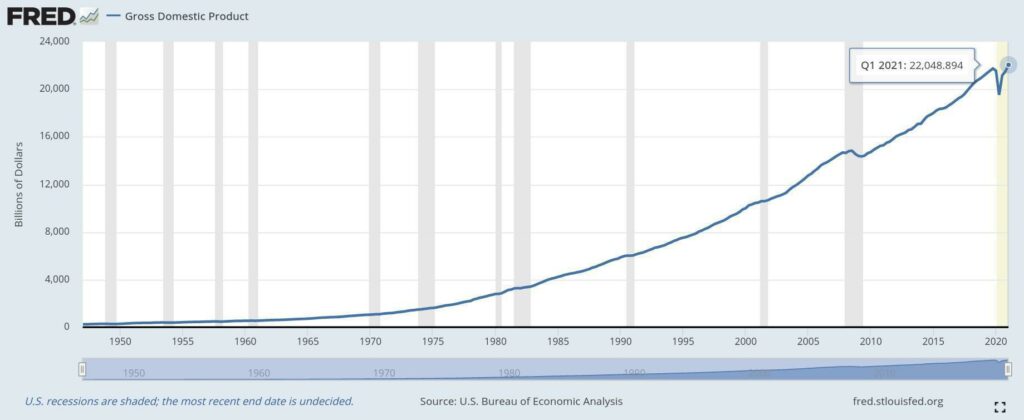
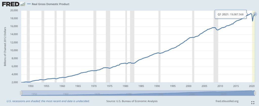
We see nominal (adjusted) GDP vs. real (unadjusted) GDP plots from the St. Louis Federal Reserve.

Nominal GDP

Real GDP

Transformations

There are multiple types of transformations. I’ll cover the most common in this post. The goal with transformations is to “transform” or remove any trend, change in variance, or seasonality — make our time series data stationary.

• Mathematical Transforms
• Difference Transforms

Mathematical Transforms

Mathematical transformations apply some function for each time series value to remove a pattern. The most common mathematical transformations are:

• Log Transformations
• Power Transformations
• More Sophisticated Transforms

Log Transformations

Converting time series data to a logarithmic scale reduces the variability of the data. Data scientists frequently use log transformations when dealing with price data. Log prices normalize the rate of change. In other words, a 10-20 move looks the same as a 100-200 move.

Let’s transform our Bitcoin data from a linear to a logarithmic scale.

import pandas as pd
import numpy as np

df1 = btc_price_history['close'].apply(np.log)
df1 = np.log(btc_price_history['close']) # equivalent
plot_chart(df1, “Bitcoin History (Log)”) # equivalent

Notice how the earlier fluctuations are now prominent, and the later price movements have less variance.

Power Transformations

Power transformations are less intuitive than logarithmic transforms. For this, we’ll create simulated data. Random exponential data is still stationary.

A trend np.square that is compounding cumsum is not stationary, as you can see in the mean and the distribution shift.

expo = pd.Series(index=dti,
    data=np.square(np.random.normal
                                        (loc=2.0,
                                         scale=1,
                                         size=periods).cumsum()))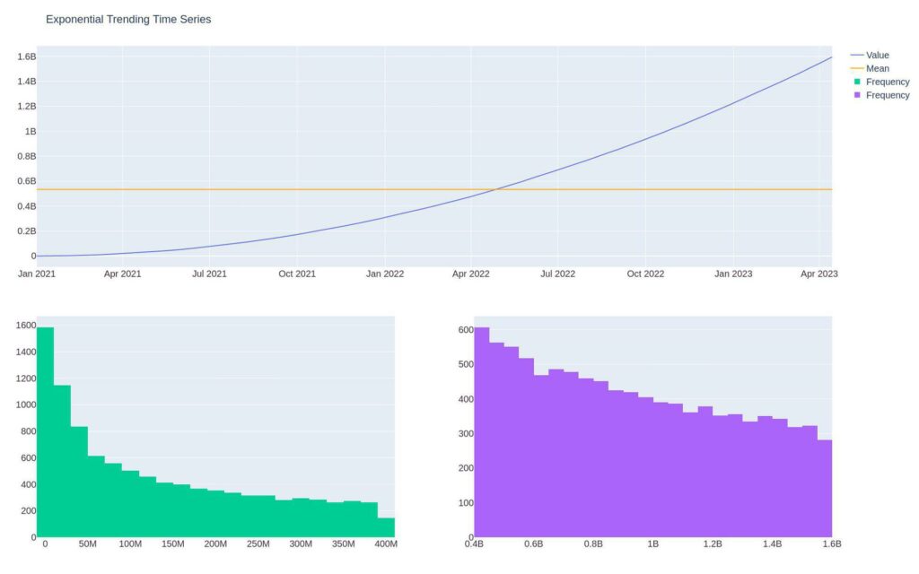

We can use the mathematic transform np.sqrt to take the square root and remove the trend using differencing, which we’ll cover shortly.

make_plot(np.sqrt(expo).diff(), "Time Series Power Transformation")

More Sophisticated Transform

The Box-Cox, Yeo-Johonson, and other power transformations attempt to transform data into a normal distribution for prediction purposes. While not always necessary for stationarity, these models often correct issues of non-linearity.

Difference Transforms

Difference transforms remove the trend or seasonality from the data.

To remove the trend, most times, you’ll perform first-order differencing.

To remove seasonality, you subtract the appropriate lagged value.

First-Order Differencing

A first-order difference is the first period minus the prior period — it’s the rate of change or returns when we’re talking about stocks.

delta y = y_t1 – y_t2

We’ve already reduced the variance from Bitcoin using a logarithmic transform. Now let’s attempt to remove the price trend using first-order differencing.

We can check for stationarity using the ADF test:

t_stat, p_value, _, _, critical_values, _  = adfuller(btc_log_diff.values, autolag='AIC')
print(f'ADF Statistic: {t_stat:.2f}')
print(f'p-value: {p_value:.2f}')
for key, value in critical_values.items():
     print('Critial Values:')
     print(f'   {key}, {value:.2f}')

ADF Statistic: -69.93
p-value: 0.00
Critial Values:
   1%, -3.43
Critial Values:
   5%, -2.86
Critial Values:
   10%, -2.57

It appears as though we were successful. The ADF statistic shows the log returns of Bitcoin are stationary. This enables us to predict the potential price of Bitcoin using models that assume stationary.

Second-Order Differencing

Second-order differences are the difference of differences or the pace of change of the rate of change.

delta delta y = delta y_t – delta y_t1

N-Th Order Differencing

While you can go to the third-order or fourth-order difference, it’s not a common practice. In most modeling scenarios, you’ll be concerned with only the first or second difference, e.g., the returns or the rate of change in the returns.

Seasonal Differencing

To subtract an annual trend, you would subtract the prior year period, such as removing last January from the current January.

A seasonal period that lasts 100 periods would subtract the 101st lag from the 1st lag.

delta y = y_t1 – y_t2

The Bottom Line

Making a time series stationary is a requirement for many prediction models. In this post, you learned many tools to create stationarity out of a non-stationary series.

We also saw that while Bitcoin price data is not stationary, the log returns are — opening up the possibility to create a mean-reverting algorithmic trading system.