Technical analysis is a methodology that uses past price and volume data to predict future prices. Here is a chronicle of the history of technical analysis and the significant events that have led to its evolution.
When we set out to analyze market movements, the two most essential tools are fundamental and technical analysis. Fundamental analysis values an asset by estimating its future discounted cash flows using the company, industry, and market information.
On the other hand, technical analysis uses historical price data and volume information to forecast market movements. Technical analysis attempts to identify market sentiment and money flow to make profitable trades.
Let us take a look at the brief history of technical analysis. Over a century’s observation of financial markets has laid the foundation of technical analysis. Many noted analysts have developed technical analysis tools, authored several books on technical analysis, and developed intricate frameworks for the technical traders to place winning bets.
Ancient History of Technical Analysis
Technical analysis has been present in primitive forms since ancient times. The book ‘The Evolution of Technical Analysis: Financial Prediction from Babylonian Tablets to Bloomberg terminals’ by Andrew W. Lo and Jasmina Hasanhodzic indicates that Assyrian trading stations in Anatolia, Turkey, or present-day Asia Minor, kept track of price fluctuations.1
Even in ancient Greek markets, speculations were an everyday affair. Merchants in Athens acknowledged that information was crucial. The book reveals that the merchants attributed particular importance to geographical and environmental data that included the most navigable trading routes and the hazards that one could meet on the way.
They made their manuals to track the developments en route. One such manual was the Periplus Maris Erythraei.2 It provided detailed information about the products sold in several countries while traveling to India and the trade policies of the rulers back then.
17th Century: Joseph De La Vega and the Dutch Market
One of the prominent indications of technical analysis in “Joseph de la Vega’s” description of the Dutch markets in the 17th century.3 Joseph de la Vega was a diamond merchant, financial expert, philosopher, and poet residing in Amsterdam during that period. His masterpiece Confusion of Confusions which he wrote in 1688, became a guiding light for modern-day technical analysis.4

Besides general investment advice, this book contains detailed descriptions of puts, calls, pools, and speculations. These are the techniques that De Vega used to predict stock price movements in the Amsterdam stock exchange.
18th Century: Homma Munehisa’s Candlestick
The oldest example of technical analysis in Asia dates back to the early 18th century. Homma Munehisa, a speculator and an early behavioral economist, developed techniques that evolved into the Candlestick, which analysts regard as the primary charting tool.5 Munehisa is also known as Sokyu Homma or Sokyu Honma and was a wealthy rice merchant and trader from Sakata, Japan. He lived during the Tokugawa Shogunate.
Munehisa described early forms of technical patterns in his book The Fountain of Gold—The Three Monkey Record of Money in 1755.6 He stated that trends and reversals are related to human emotions, reflecting market behavior. In Japan, candlestick charts are called Sakata charts, named after Homma’s native place.
In Edo-period Japan, traders used technical analysis to profit from Osaka’s rice futures market. Some of the candlestick chart patterns which the traders then used were “Night and morning attacks”; “advancing three soldiers”; and “counter attack lines.”
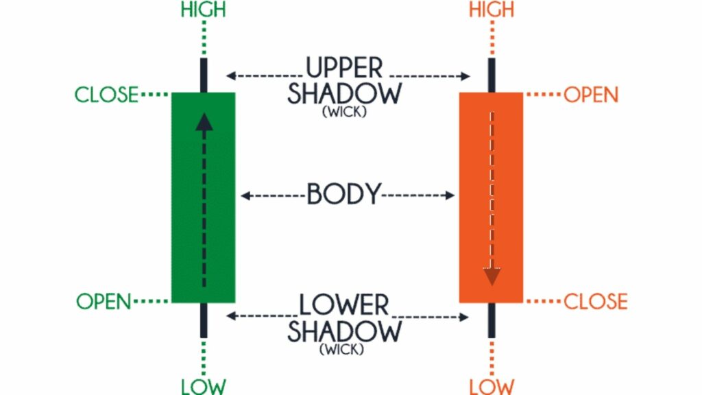
Candlestick charts use open, high, low, and close price data and are drawn in a way that resembles a candle with wicks on both ends. The high and low are described as shadows and plotted as a single line.
Initially, only physical rice trading was done in Japan, but since the beginning of 1710, a futures market was established where coupons represented future rice delivery. Homma flourished as a trader in this secondary market of trading rice coupons. Recognized for his ability as an expert trader in the rice market, Homma also became a financial advisor to the government. It also awarded him the rank of honorary Samurai.
On the other side of the East China Sea, the rules established by Confucian manuals helped forecast price movements in the markets of Imperial China.7 One such manual, Essential Business, elaborated that “no item will remain expensive for over one hundred days and no item will remain cheap for one hundred days.” The same manual also showed merchants how to identify market movements and understand associations between price movement and volume.
1896: The Dow Theory by Charles Dow
After developing the Dow Theory, the technical analysis came to the US in the late 19th/early 20th century. The Dow Jones & Company co-founder, Charles Dow, pioneered the Dow Theory. He also founded the company Edward Jones and Charles Bergstresser in 1896.8 The theory has evolved throughout the decades and forms the basis of the present-day technical analysis.
Charles Dow closely analyzed American stock market data and published some of his findings in The Wall Street Journal editorials. He looked for patterns and business cycles that could be found through a “Dow Theory.” The Dow theory states the market is upward if one of its averages advances above a previous necessary high and if another average also follows a similar advance. Dow recorded the highs and lows of his daily, weekly, and monthly trades and studied the patterns of the market’s peaks and troughs.
Charles Dow passed away in 1902 because of which he could not publish his complete theory on the markets. However, he had several followers who published his works and conducted further research on the editorials over the next century. This includes significant contributions by William Hamilton, Robert Rhea, E. George Shaefer, and Richard Russell in the 1960s, which we will discuss in detail later.
1920: Ichimoku Kinko Hyo
Ichimoku Kinko Hyo was a charting technique that a Japanese journalist, Goichi Hosoda, developed in the 1920s.11 Hosoda was also known as Ichimoku Sanjin, which means “what a man in the mountain sees.” He spent over 30 years fine-tuning the technique before finally releasing it to the public in the late 1960s. Most people also believe that he employed over 10,000 university students to backtest the indicators that laid the foundation of the Ichimoku trading method. Ichimoku is built on candlestick charting to enhance the accuracy of forecasting price movements.

Ichimoku is a moving average-based trend analysis tool with more data points than standard candlestick charts. This is why it provides a clearer picture of potential price action. The primary difference between the plotting of moving averages and that of Ichimoku is that Ichimoku’s lines use the 50% point of the highs and lows instead of the candle’s closing price.12
Hosoda claimed that the traders could determine momentum, support, and resistance by looking at the chart in just one glance. “Ichimoku” in Japanese means “one look,” hence the name. Not only this, Ichimoku allows traders to assess price action across three time frames – long, medium, and short. This technical indicator consists of the tenkan-sen, kijun-sen, senkou span A, senkou span B, and chikou span.
In 1969, when Hosoda finally presented his book to the Japanese public, it became the nation’s most popular and widely-used indicator. Ichimoku depicts the entire market story, including trade direction, primary support, and resistance lines. You can also find the specific entry and exit points. The Ichimoku is so versatile that it can be used across all markets and time frames.
Hosoda was far-sighted and firmly believed that the market directly reflected the dynamics of collective human behavior. He assumed that human behavior was always in a constant cyclical movement and swayed back and forth from the equilibrium and interactions. Each of the five components that are a part of Ichimoku reflects such an equilibrium.
Even as the Ichimoku was massively popular across Asia, it only appeared in the Western world in the 20th century. However, it still wasn’t well-accepted, and many traders failed to understand its appeal.
1929: William Hamilton Refines Dow Theory
William Hamilton succeeded Charles Dow as the Editor of The Wall Street Journal and authored a famous editorial, “A Turn in the Tide” on October 25, 1929. He drew a significant conclusion in his editorial, which said, people are trading on Wall Street, and many all over the country have never seen a real bear market…. What is more material is that the stock market does forecast the country’s general business. The big bull market was confirmed by six years of prosperity, and if the stock market takes the other direction, there will be a contraction in business later…” 10
Hamilton worked actively to refine the Dow Theory between 1902 and 1930. In 1922, he also wrote The Stock Market Barometer to explain the theory.9 The Dow Theory could not predict the extent or duration of these changes, but it could predict their occurrence.
Hamilton explained the Dow Theory by establishing a metaphor between market trends and ocean waves. The long-term trend of four years or more was referred to as the tide of the market, which could be rising, which is bullish, or falling, which is bearish. Market trends that lasted a week or a month were the shorter-term waves. Lastly, the day-to-day fluctuations were like sporadic water flashes in the rough ocean.
Besides these techniques, Hamilton used the railroad and industrial averages as barometers of market trends. The direction of these averages indicated the bull and bear market with accuracy. If both Dow Jones averages are marching in the same direction, it applies to the entire market. Overall, the Dow Theory analyzes the behavior of market trends in detail. The theory signals to identify the underlying market trend and place trades based on that.
1930: The Elliott Wave Theory
In 1930, American accountant, author, and investor Ralph Nelson Elliott developed the Elliott Wave Theory.13 Elliott was deeply Inspired by the Dow Theory and found that traders can predict the stock market movement by studying and identifying a repetitive pattern of waves.
Elliott analyzed the markets, identified wave patterns’ specific traits, and made elaborate predictions based on the patterns. A portion of his work drew inspiration from the Dow Theory, which studied price movements in the form of waves. However, Elliott also identified the “fractal” nature of markets and was intrigued by the recurring geometric patterns of price movements during a particular time frame.
He diced the patterns and studied them in greater detail. Elliott then discovered that even stock index price patterns followed a similar arrangement. Fractals are mathematical elements that tend to repeat themselves constantly on a smaller scale.14
Elliott’s wave theory, or Elliot’s take on technical analysis, was first published in The Wave Principle in 1938. Elliott firmly believed that though stock markets are highly unpredictable and volatile, they traded in repetitive patterns. The Elliott Wave Theory looks for recurrent long-term price patterns resulting from constant investor sentiment and psychological changes. Each set of waves belongs to a more extensive set of waves that resonate with the recurrent pattern. Elliott proposed that the stock price trends reflect the deeper psychology of investors. He also concluded that the ups and downs in investor psychology are reflected in the “waves” or the recurring fractal patterns.
1932: Robert Rhea – Dow Theory
In 1932, Robert Rhea, an avid investor, refined Hamilton’s analysis and took the Dow Theory to the next level. He conducted in-depth studies and decoded over 200 editorials written by Charles Dow and William Hamilton.9
Rhea also referred to Hamilton’s The Stock Market Barometer and used his research and studies to form theorems and hypotheses to author a book called The Dow Theory. Rhea, a prime proponent of the Dow Theory, publicized its use as a practical tool for taking long and short positions in the market. He also pointed out the tops and bottoms of the market and earned profits from his calls.15
He called the market bottom in 1932 and a top in 1937 in his newsletter, the Dow Theory Comments. The calls led many subscribers to earn massive profits and consequently brought in more subscribers.
1935: Gann Angles by William D. Gann
In 1935, William Delbert Gann, a finance trader, developed technical analysis methods like the Gann angles and the Master Charts.16 Master Chart is a collection of various tools Gann created, such as the Spiral Chart, the Circle of 360, and the Hexagon Chart.
Gann built his forecasting methods primarily around geometry, astrology, and astronomy. In his 1935 book, The Basis of My Forecasting Method, he propagated angles in the stock market. Gann angles focus around a 45-degree angle, also called the 1:1 angle, and are applied from price bottoms on their way up or from the price tops on their way down.
Gann considered the 45-degree angle the perfect balance between the price movement and time. The price trends above it are strong, and below that, one is weaker. Some of the other Gann angles include 2:1, 3:1, 4:1, 8:1, 1:2, 1:3, 1:4, 1:8. The crux of the theory is that if the price moves through a particular angle, it will move towards the next. In the real-life scenario, a trader can tweak the ratio according to their trades, provided they maintain consistency.
1948: Robert D. Edwards and John Magee
In 1948, Robert D. Edwards and John Magee published Technical Analysis of Stock Trends, one of the most influential works in technical analysis.17
The work focuses exclusively on trend analysis, volume analysis, and chart patterns used to this date. This book by Edwards and Magee is one of the first in-depth works on technical analysis. It produced a framework for deciphering investors’ and markets’ repetitive and predictable behavior.
Not only this, but the book also dissected the Dow Theory in finer detail. The book laid the foundation for modern technical analysis. It brought several concepts such as head and shoulders, triangle tops, bottoms, double tops, support, resistance, and trend lines. The original edition has been revised close to nine times until now.
1949: Donchian Channels
In 1949, Richard Donchian was the first to formulate diversified strategies based on five- and twenty-day moving-average crossovers. His significant discovery was the Donchian channel, and he also founded Futures Inc, the first public managed futures fund. Donchian Channels are three lines that the moving average calculations generate.
It is an indicator created by upper and lower bands around a median band. The upper band indicates the highest security price over a set number of periods, while the lower band indicates the lowest price over a particular number of periods. The area that lies between the upper and lower bands is the Donchian Channel.18
Donchian channels depict critical elements like volatility, breakouts, and potential overbought/oversold conditions for a security. When used in combination with other technical indicators, the upper and lower bands of a Donchian channel can also form effective support and resistance levels.
Richard Donchian formed a four-week rule and allowed the markets to determine their own bands through this rule. The four-week rule entails that a buy signal happens if the price moves past the 4-week high, and if the price drops below the 4-week low, it’s a sell signal. Eventually, connecting the 4-week highs and the 4-week lows through this rule forms an envelope.
1950: Stochastic Oscillator
In 1950, George Lane, a securities trader, educator, and an active member of the group of futures traders in Chicago, developed the Stochastic Oscillator. A stochastic oscillator is a momentum indicator that compares a particular security’s closing price to a range of price points over a specific period. The closing price sometimes ends near the high in an uptrend and towards the low in a downtrend. However, If the closing price moves away from the high or the low, it indicates a slowing momentum.19
Since Stochastic oscillators depend on the historical prices of the asset, they could vary around some mean price level. %K is the “fast” stochastic indicator, while %D is the “slow” one. %D is the 3-day moving average of %K.
The K% denotes the closing price in relation to its price range over 14 days. A k% of 80% indicates that the price closed above 80% of all the previous closing stock prices over the past 14 days.
Lane described the origins of the %K and %D stochastic oscillator as follows:
“We developed %A but found that it didn’t work. We went on to research and followed 28 oscillators. As we progressed through the oscillators we were developing; we expressed them as percentages; thus: %D, %K, %R, etc. We pioneered using the computer to test our oscillators.” 20
George Lane believed that the Stochastics indicator is best used with other techniques and indicators such as Elliott Wave Theory, cycles, and Fibonacci retracement for the perfect timing. A core point of Lane’s theory is the divergence and convergence of trendlines plotted on stochastics.
However, the credit for Stochastics Oscillator’s development doesn’t lie with George Lane alone. While Lane popularized the indicator, C. Ralph Dystant also had a critical role in originating it. In 1948, Dystant operated a school called Investment Educators, which offered courses in stock market trading. Many believe that he introduced the Stochastic Oscillator as a part of his Elliott Waves Course.21
1960: Exponential Moving Average
In the early 1960s, PN (Pete) Haurlan developed the Haurlan Index. It is a technical indicator that ascertains market breadth to short, intermediate, and long-term timeframes with moving averages based on the daily Advance-Decline (A-D) difference. Today, only a handful of professional technical analysts use the Haurlan Index. However, it generated a lot of buzz when first introduced in the 1960s.23
P.N. Haurlan also introduced exponential moving averages to track the price patterns in the financial markets in 1960. Haurlan was a rocket scientist working for the Jet Propulsion Laboratory in Pasadena, California, in the early 1960s, and he borrowed the mathematical concept of EMA from his rocketry days.
EMAs were used in designing analog tracking circuitry because of their simplistic nature. For calculating a 50-day simple moving average, one must track the last 50 data points, which was too cumbersome for the formative computers. On the other hand, while calculating the EMA, the computer only requires the current data value, the smoothing factor to be applied, and the previous EMA value.24
1960: Moving Average Convergence Divergence
In the 1960s, Gerald Appel created the MACD or the Moving Average Convergence / Divergence. MACD is a powerful technical indicator that shows the difference between a fast and slow exponential moving average (EMA) of closing stock prices.22 The standard periods that Gerald Appel recommended in the 1960s are 12 and 26 days. The 12-day EMA is the faster one, while the 26-day is slower.
An exponential moving average (EMA) is a moving average (MA) that allocates more weightage to the most recent data points. The MACD line can indicate changes in stock trends by drawing comparisons between EMAs of different periods. An analyst can detect minor changes in the stock’s trend while comparing the difference between a fast and slow EMA to an average. On the MACD chart, a nine-day EMA of the MACD is also plotted for buy and sell decisions.
MACD helps investors understand the strength or weakness of the trends in the price-bullish or bearish. MACD also triggers technical signals when it crosses its signal line upwards or downwards. These crossovers’ pace is also a signal to gauge whether a market is overbought or oversold.
The 1960s: The Beginning of Bands and Envelopes
Bands, envelopes, and channels enjoy a critical place in technical analysis and have an exciting history. It is known as an envelope when the trend lines are built over and above the current price. A simple moving average usually generates an envelope’s upper and lower bands at a prescribed distance above and below the moving average. The direction of the envelope depends on the direction of the moving average.
One Of The Earliest Mentions Of The Envelope Is Wilfrid Ledoux’s Twin-line Chart, Which He Copyrighted In 1960. These Lines Are Connected Monthly Highs With A Black Line And The Monthly Lows With A Red Line. When The Red Line (Monthly Lows) Surpassed A Trough Made By The Black Line (Monthly Highs) By Two Points, It Signified A Buy Signal.25,26
Around the same time, Chester W. Keltner mentioned the Ten-Day Moving Average Rule in his book, How to make money in commodities, also known as Keltner channels.26
Keltner calculated the typical price by taking the average of the High, Low, and Close points (H+L+C)/3 and calculating the 10-day moving average of the price centerline. The lines above and below are plotted at a specific distance from the centerline. This distance is nothing but a simple 10-day moving average. A close above the upper line is a strong bullish signal, while a close below the lower line is seen as a strong bearish sentiment.
1967: TRIN Index by Richard Arms Jr.
In the 1967s, Richard Arms Jr. developed The TRIN or the TRading Index. It is also known as the Arms index. A short-term trading indicator based on the Advance-Decline Data.26 compares the number of advancing and declining stocks (AD Ratio) to advancing and declining volume (AD volume). A value below 1 indicates bullish sentiment, and a value above 1 – is bearish. TRIN is continuously displayed on the New York Stock Exchange’s central wall display during trading hours.
It serves as a predictor of future price movements in the market, primarily on an intraday basis. It does this by generating overbought and oversold levels, which indicate when the index (and the majority of stocks in it) will change direction. A TRIN reading above typically accompanies a substantial price decline since the strong volume in the decliners helps fuel the selloff.
1969 – McClellan Oscillator and Summation Index
Sherman McClellan, and his wife Marian, created the McClellan Oscillator and Summation Index. The Oscillator is an indicator for market breadth, calculated as a difference between declining issues and the number of advancing issues.27
The objective behind the McClellan Summation Index was to identify bullish or bearish trends and their strength. The McClellan Oscillator offers various structures, but there are two primary ones. First, when the Oscillator is positive, it usually denotes the inflow of money into the market; on the other hand, it depicts an outflow of money when it is negative. The second interpretation says, when the Oscillator reaches extreme readings, it can denote an overbought or oversold condition.28
When all the daily values of the McClellan Oscillator are added, it produces an indicator known as the McClellan Summation Index. It forms the basis for intermediate and long-term interpretation of the stock market’s direction and its impact. The Oscillator usually moves between 0 and +2000.
1970: Introduction to Cycles
Between 1960 and 1970, JM Hurst, an American engineer, became the first researcher to use the power of technology to study cycles in the financial markets.29 JM Hurst is the ‘father’ of modern cyclic analysis. In January 1970, J.M Hurst published The Profit Magic of Stock Transactions. In the book, Hurst presented the “constant width curvilinear channels” to highlight the cyclic nature of the stock price changes.
A workshop-style course called the Cyclitec Cycles Course followed the book’s publication. The course was also known as “JM Hurst’s Cycles Course.” He presented the Cyclic Theory in both these works, after which it became really popular. The Profit Magic book also mentioned a technique for applying his Cyclic Theory. However, he presented his work in more detail in his Cycles Course.
1970: Establishment of the CMT Association
Even with much development in charting and various innovative tools, technical analysis was still seen as an obscure concept. A significant development in 1970 was the establishment of the Market Technicians Association (MTA).37This organization was set up by professional technical analysts who sought to make Technical Analysis a widely accepted discipline in market research and prediction. Many of the MTA members are renowned and high-authority analysts with extensive authorship.
The Association for Chartered Market Technicians, or CMT, was officially founded by Ralph Acampora, John Brooks, and John Greeley. It started in New York as an informal meeting of professional technical analysts and originally had 18 members. In 1973, the CMT Association was established as a not-for-profit association.
Today, there are several Professional technical analysis societies across the world. Society of Technical Analysts (STA) represents it in the UK, while in Canada, the representative body is called the Canadian Society of Technical Analysts.
1978: Relative Strength Index
Developed by J. Welles Wilder Jr. in 1978, the Relative Strength Index (RSI) is a momentum oscillator for measuring price movements and speed changes.30 Wilder first discussed the concept in his1978 book, New Concepts in Technical Trading Systems. This book also features Parabolic SAR, Average True Range, and the Directional Movement Concept (ADX). RSI was also featured in the June edition of Commodities magazine.
Like the McClellan indicators, Wilder’s indicators offered detailed explanations of using daily worksheets and manually calculating the formulas behind indicators. All these indicators by Wilder Jr. are early instances of thinking beyond the immediate price action.32
J. Welles Wilder, Jr. was an American mechanical engineer turned realtor. However, he left the real estate business in 1972 and began trading in the commodities market. He devoted a lot of time developing mathematical concepts and creating efficient trading mechanisms in highly leveraged assets.31
According to Wilder Jr., RSI moves between zero and 100 and is considered overbought when it moves above 70 and oversold when it goes below 30. RSI is also helpful in identifying the general trend.
1980: Jim Yates and the Zone System
In the early 80s, Jim Yates, an expert options trader and the co-founder of the CBOE Options Institute, propagated the concept of analyzing bands in relation to volatility.33 He conceived a The Zone System that employed the Implied volatility from the options market to make informed investment decisions.
The Zone system analyzes the stock price’s deviation from its trend. These are the six areas under a normal distribution curve where each had a specific execution strategy.34 Zone 1 represents the area between two and three standard deviations below the mean, while another extreme is Zone 6. These zones are the farthest points from a stock’s mean, the vertical line dividing the normal curve. It is also called the trend. The two-time frames chosen for analysis were ten days and 90 days, which is ideal for a short-term trader and options hedger.
The objective of the zone system was to determine if an asset was overbought or oversold in relation to the price and volatility.
1980: The Development Of Bollinger Bands
John Bollinger, an options trader in the 1980s, met Mr. Yates and was deeply impressed by his idea. He wanted to introduce adaptive trading bands because he concluded that volatility was a dynamic concept instead of the common belief being static.35
He devised a way to automate the breadth of the channel that Yate’s Zone system formed. Thus, Bollinger based the band’s spread on the current average volatility. He believed that this was a better way to form bands because there existed a direct link between the volatility and the standard deviation of prices. He named these tools Bollinger bands.
Bollinger Bands can be used across time frames, ranging from short-term to hourly, daily, weekly, or monthly. It can also be applied to all asset classes such as equities, forex, commodities, and futures.
1986: Histogram Added to MACD
In 1986, Thomas Aspray added the divergence histogram or bar graph to the MACD indicator. The objective behind the MACD histogram is to anticipate MACD crossovers.36 This is an important indicator to assess critical price movements in the underlying security. The MACD-Histogram is critical in measuring the distance between the 9-day EMA of MACD and the MACD itself.
The MACD-Histogram, just like MACD, oscillates below and above the zero line. Being a moving average, MACD lags price, and there can be a delay in signal line crossovers impacting the reward-to-risk ratio. The divergences in the MACD Histogram-Bullish or bearish can signal chartists that a crossover in the MACD signal line is round the corner.
If the MACD is above the signal line, the MACD histogram will be above the MACD’s baseline and vice versa. Traders use the MACD’s histogram to understand the impact of the bullish or bearish momentum.
1991:Candlestick Charts in the US
Steve Nison introduced the Japanese Candlesticks to the Western world with his 1991 book, Japanese Candlestick Charting Techniques. He was who was among the first to receive the Chartered Market Technician (CMT) designation after its introduction in 1989.39
2005: The SEC Recognizes CMT Charter
In 2005, the Financial Industry Regulatory Authority (FINRA) appealed to the Securities and Exchange Commission to accept the CMT Program levels 1 and 2 exams in place of the Series 86 examination required of financial analysts.37
Previously, the Securities and Exchange Commission (SEC) always portrayed a strong stance against chart-based methods and firmly believed only in fundamental analysis.38
However, in 2005, SEC amended Rule 344 and allowed the CMT charter recognition for technical analysts. According to the amended rule, officially, two separate categories of Wall Street research analysts would exist- a fundamental analyst with a CFA diploma; and a technical analyst who has a CMT diploma.
The Bottom Line
Technical analysis has existed since ancient times, but it was only between 1960 and 1970 that the primary tools and techniques used in modern-day technical analysis were developed. The landscape of technical analysis and stock trading, in general, changed after the advent of the internet.
In recent years, the proliferation of algorithmic trading has brought in a whole new bunch of traders who rely purely on technicals and statistics, with minimal emphasis on psychological elements. From being seen as an obscure predicting mechanism to one of the most widely accepted forms of market analysis, technical analysis has come a long way.
Sources: 1, 2, 3, 4, 5, 6, 7, 8, 9, 10, 11, 12, 13, 14, 15, 16, 17, 18, 19, 20, 21, 22, 23, 24, 25, 26, 27, 28, 29, 30, 31, 32, 33, 34, 35, 36, 37, 38, 39